Raman spectroscopy (spontaneous, gas phase)

Summary

Shine a laser into a jar of gas and almost all of the light either passes straight through or bounces off unchanged. But a tiny fraction — roughly one photon in a billion — bounces off with its color very slightly shifted, because it briefly nudged a gas molecule into vibrating or spinning and left a little energy behind (or picked a little up).

That color shift is different for every kind of molecule, so measuring it tells you, from a single laser shot, exactly which gases are present and roughly how much of each — hydrogen, methane, carbon dioxide, nitrogen, and hydrogen sulfide all show up as separate, non-overlapping peaks in the same spectrum. This matters for hydrogen specifically because H₂ is invisible to the workhorse infrared gas sensors (it has no electrical “handle” for infrared light to grab), so Raman is one of only two optical techniques that can see it directly at all.

The same “one photon in a billion” weakness returns: at the parts-per-million levels typical of a promising soil-gas sample or of ordinary background air, that already-rare scattered photon becomes vanishingly rare, and a real commercial Raman gas analyzer today can reliably see hydrogen down to only a couple thousand parts per million, far too high for soil-gas exploration.

Where the technique already works well, and is sold as a mature off-the-shelf product, is measuring concentrated gas streams: pipelines, industrial process gas, and turbine fuel blends where hydrogen sits at the percent level. For Hestia, this is the wrong tool for finding a hydrogen seep in the ground, but a genuinely excellent, already-commercial tool for confirming hydrogen content in a flowing, pressurized gas stream once one is found.

Note

Context numbers used throughout this page: atmospheric H₂ background ≈ 0.53 ppm; geologic H₂ soil-gas anomalies span roughly 1 ppm to percent level [11]; H₂ LEL = 4 vol% (40,000 ppm). This page covers spontaneous, linear, gas-phase Raman only — the same scattering mechanism boosted by cavities, hollow-core fibers, plasmonics, or coherent (CARS/SRS) multi-wave-mixing is a physically distinct engineering problem, covered on the Enhanced Raman page.

At a glance — published performance envelope

Detection limit

190–2,100 ppm

Range

190–1,000,000 ppm

Response t₉₀

1–900 s

Recovery

1–600 s

Selectivity

high

Drift

low

Operating T

−20 … 150 °C

Humidity

0–90 % RH

Power

150 mW – 300 W

Unit cost

$20k–$200k

TRL

9

Main interferents: CH₄, CO₂, N₂, CO · poisons: none, optical fouling. Ranges span the published devices/variants covered below — per-claim citations are in the body; data: src/data/modalities/raman-spectroscopy.yaml.

Mechanism & physics

Why Raman sees H₂ when infrared cannot

H₂ is a homonuclear diatomic molecule: it has no permanent dipole moment, and stretching the bond does not create one to leading order, so the fundamental rovibrational transitions that dominate infrared absorption for heteronuclear molecules are dipole-forbidden.

This fact shapes essentially every sensing technology in this compendium: H₂ offers very few physical handles, and Raman scattering exploits one of the only two optical ones available (the other being deep-UV electronic transitions in the Lyman/Werner bands below ~112 nm, unusable in ambient air; see UV/EUV and fluorescence).

Raman scattering does not require a permanent or transition dipole; it requires that the molecule’s polarizability change during the nuclear motion. An oscillating electric field $E = E_0\cos(\omega_0 t)$ (the laser) induces a dipole moment $\mu_{ind} = \alpha\,E$ in the molecule.

For a vibrating/rotating molecule, the polarizability is itself modulated at the vibration/rotation frequency, $\alpha(t) = \alpha_0 + \left(\dfrac{\partial \alpha}{\partial Q}\right)_0 Q(t) + \dots$, where $Q(t) = Q_0\cos(\omega_{vib}t)$ is the normal-mode coordinate. Substituting produces three frequency components in the induced dipole’s oscillation: the elastic (Rayleigh) term at $\omega_0$, and two inelastic (Raman) sidebands at $\omega_0-\omega_{vib}$ (Stokes) and $\omega_0+\omega_{vib}$ (anti-Stokes).

H₂’s bond polarizability changes strongly with internuclear separation and is anisotropic (easier to polarize along the bond axis than across it), so H₂ is a strong Raman scatterer despite being completely IR-dark — the textbook mutual-exclusion complementarity of Raman and IR selection rules for centrosymmetric molecules. This is why every gas-phase Raman analyzer vendor markets the technique as “the one optical method that sees H₂, N₂, and O₂ directly” [1][2].

Selection rules and line positions

The rigorous treatment is Placzek’s polarizability theory. The gross selection rule for rotational Raman activity is that the polarizability must be anisotropic (trivially true for any diatomic); the specific selection rule for a linear molecule in a $\Sigma$ electronic ground state is

$\Delta J = 0, \pm 2$

with $\Delta J=+2$ giving the Stokes-side S-branch (the practically important one) and $\Delta J=-2$ the anti-Stokes O-branch — distinct from the IR/microwave rotational rule $\Delta J = \pm 1$, which requires a permanent dipole and so is inapplicable to H₂ at all.

For the vibrational fundamental the rule is $\Delta v = \pm 1$ together with $\Delta J = 0, \pm 2$, giving O-, Q-, and S-branch structure; for H₂ the $\Delta J=0$ Q-branch carries the overwhelming majority of vibrational Raman intensity and appears as a tight cluster of nearly coincident lines rather than a resolved branch, because the vibration–rotation interaction constant is small.

H₂’s reduced mass is the smallest of any neutral diatomic, so its rotational constant, $B_0 \approx 60.8\ \text{cm}^{-1}$ (≈164 µm equivalent), dwarfs N₂’s ($B_0\approx2.0\ \text{cm}^{-1}$, ≈5 mm), so H₂’s rotational Raman lines are widely and cleanly spaced, unlike N₂’s or O₂’s closely bunched, largely unresolved rotational wings.

The two lowest, most diagnostic S-branch lines are S₀(0) ($J=0\to2$, para-H₂, even $J$), Raman shift ≈354 cm⁻¹ (scattered at ≈542 nm with a 532 nm pump), and S₀(1) ($J=1\to3$, ortho-H₂, odd $J$), ≈587–588 cm⁻¹ (≈549 nm) and the strongest rotational line in a room-temperature sample [2][3].

H₂’s nuclear-spin statistics (the proton is a spin-½ fermion) split the population into ortho-H₂ (nuclear-spin triplet, odd $J$ only) and para-H₂ (nuclear-spin singlet, even $J$ only) with a 3:1 statistical weight at thermal equilibrium — why S₀(1) and the vibrational Q₁(1) line dominate a room-temperature spectrum, a fingerprint ORNL researchers explicitly confirmed matches reported gas-phase spectra [2].

The vibrational Q-branch near 4,100–4,160 cm⁻¹ (a 2.44–2.40 µm vibrational quantum; scattered at ≈680–683 nm with a 532 nm pump) is in practice a comb of closely spaced lines rather than one sharp feature, because the vibrational frequency depends weakly on rotational state $J$:

Line	Assignment	Raman shift (cm⁻¹)	Scattered λ (532 nm pump)
Q₁(0)	v: 0→1, para-H₂, J=0	≈4,161	≈683.3 nm
Q₁(1)	v: 0→1, ortho-H₂, J=1 (dominant, ~3:1 weight)	≈4,155–4,157	≈683.0–683.1 nm
Q₁(2)	v: 0→1, para-H₂, J=2	≈4,143	≈682.4 nm
Q₁(3)	v: 0→1, ortho-H₂, J=3	≈4,126	≈681.6 nm

ORNL’s own commercial-instrument spectra (Kaiser Rxn2, 532 nm) directly resolved Q₁(1)/Q₁(2)/Q₁(3) near 4,157 cm⁻¹ and the S₀(0)–S₀(3) rotational ladder at ≈588, 756, and 1,039 cm⁻¹ (scattered ≈549–563 nm) [2], closely matching independently reported simulation values of 357/592/819/1,039 cm⁻¹ and measured values of 588 cm⁻¹ (rotational) / 4,155 cm⁻¹ (vibrational) [2][3].

For field spectroscopists, H₂ occupies two clean, uncrowded spectral windows: a low-wavenumber rotational window (300–1,100 cm⁻¹, scattered at ≈541–565 nm for a 532 nm pump, shared territory with N₂’s weak rotational wing and dust/window Rayleigh leakage) and a high-wavenumber vibrational window (4,100–4,200 cm⁻¹, scattered at ≈680–685 nm) that is essentially unoccupied; no other common exploration-relevant gas (CH₄ ≈2,917 cm⁻¹, CO₂ ≈1,285/1,388 cm⁻¹ Fermi dyad, N₂ ≈2,330 cm⁻¹, CO ≈2,143 cm⁻¹, H₂S ≈2,611 cm⁻¹ — for a 532 nm pump, all scattering between ≈571 and 630 nm, well short of H₂’s Q-branch at ≈683 nm) puts a fundamental anywhere near it.

This uncrowded window is a major practical reason H₂ is comparatively easy to identify by Raman even though it is hard to see at trace levels (below).

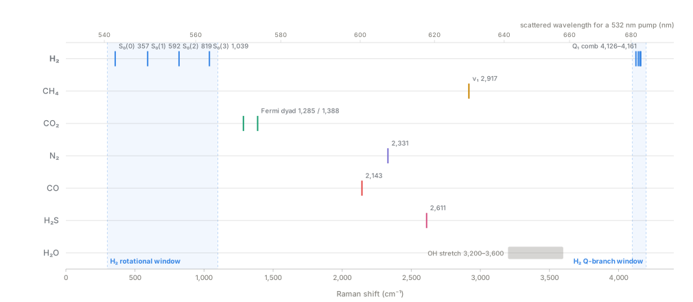
H₂’s two uncrowded windows, drawn to scale: no common co-evolved gas puts a fundamental near the S-branch window (300–1,100 cm⁻¹) or the Q-branch window (4,100–4,200 cm⁻¹). Top axis: where each line lands as scattered light with a 532 nm pump.

shift ν̃ cm⁻¹

as an absolute transition (λ = 10⁴/ν̃)
as a Raman shift: Stokes-scattered λ at this pump

1/λ_s = 1/λ_pump − ν̃. Only spectroscopic positions convert to wavelengths — absorption coefficients and NEA values quoted in cm⁻¹ are inverse path lengths, not photon energies (see the glossary "Wavenumber" entry).

Cross sections and the photon-count problem

The differential Raman scattering cross section $d\sigma/d\Omega$ (cm²·sr⁻¹·molecule⁻¹) sets the absolute photon budget. For a specific rovibrational transition, the cross section can be written in Placzek–Teller form as

$Q_S(v_i,J_i;v_f,J_f) = \frac{128\pi^5}{9\,\lambda'\lambda^{3}}\, b_{J_i J_f}\, \left|\langle R_i|\gamma(r)|R_f\rangle\right|^2$

where $\lambda'$ is the incident and $\lambda$ the scattered wavelength, $b_{J_iJ_f}$ is the Placzek–Teller rotational line-strength factor, and $\gamma(r)$ is the polarizability-anisotropy matrix element [4]. The key structural feature is the $(\lambda'\lambda^3)^{-1}$ — roughly $\nu^4$ — frequency dependence: Raman scattering, like Rayleigh scattering, is far stronger in the blue/green than in the red/NIR.

The measured absolute numbers are what matter for engineering.

• H₂’s total differential Raman cross section at 532 nm, from a laboratory Raman-lidar calibration, is $(2.70\pm0.43)\times10^{-30}\ \text{cm}^2\text{sr}^{-1}$ [5].
• Early absolute measurements at 480.0 and 514.5 nm were made by Cohen et al. (1972) [6], and the widely cited Schrötter & Klöckner (1979) review tabulates H₂’s Raman cross section as roughly 2.2× that of N₂ at 514.5 nm [7].
• The most complete modern first-principles dataset comes from Singor, Scarlett, Zammit, Bray & Fursa (2024), who computed 9,582 rovibrational Rayleigh and Raman cross sections, depolarization ratios, and reversal coefficients across H₂’s full $X^1\Sigma_g^+$ ground state, published openly on Zenodo [4].

That same work notes the vibrational Q-branch cross section is only ~1.4% of the calculated Rayleigh cross section at the same wavelength — even the “strong” H₂ Raman line is roughly two orders of magnitude weaker than ordinary elastic scattering from the same molecule [4].

For comparison, typical resonance-free electronic-absorption cross sections used in TDLAS/NDIR proxy-gas sensing run $10^{-19}$–$10^{-21}$ cm²/molecule — Raman’s $10^{-30}$ cm²/sr differential cross section is roughly 9–11 orders of magnitude smaller. This is why spontaneous Raman is a weak-signal technique, and why every commercial gas-phase Raman instrument is built to collect as many photons as possible: large lasers, tight collection optics, waveguide/fiber tricks, or long integration times.

Explicit photon-budget arithmetic

Take a representative scenario: 1 ppm H₂ in 1 atm air, a 100 mW 532 nm laser, and a realistic gas-Raman collection numerical aperture of NA ≈ 0.22 (typical multimode-fiber probe NA used in commercial Raman gas probes [8][9]).

Photon flux. Photon energy at 532 nm is $E_{ph} = hc/\lambda \approx 3.74\times10^{-19}$ J, so at 100 mW the laser delivers $\Phi_L = P/E_{ph} \approx 2.68\times10^{17}$ photons/s.

Number density. At $T\approx296$ K, 1 atm, ideal-gas total number density is $n_{tot}\approx2.5\times10^{19}\ \text{cm}^{-3}$. At 1 ppm, $n_{H_2}\approx2.5\times10^{13}\ \text{cm}^{-3}$.

Collection solid angle. For NA = 0.22, $\Delta\Omega \approx \pi\,NA^2 \approx 0.15$ sr.

Path length. Assume $L=1$ cm, typical of a focused free-space probe volume or a short flow cell — the softest assumption here, and exactly the lever every enhanced-Raman variant pulls (see Enhanced Raman).

Photons Raman-scattered into the collection cone per second, using the measured 532 nm cross section of $2.7\times10^{-30}\ \text{cm}^2/\text{sr}$ [5]:

$\dot N = \Phi_L \cdot n_{H_2} \cdot \frac{d\sigma}{d\Omega} \cdot \Delta\Omega \cdot L \approx (2.68\times10^{17})(2.5\times10^{13})(2.7\times10^{-30})(0.15)(1) \approx 2.7\ \text{photons/s}$

Even before subtracting real-world optical losses (notch/edge filter transmission, grating efficiency, mirror/lens losses, detector quantum efficiency — typically another combined factor of ~0.3–0.5), the idealized photon-generation rate for 1 ppm H₂ at 1 atm with a 100 mW laser is of order 1–3 photons per second.

A TE-cooled dispersive-spectrometer CCD, with dark current suppressed by cooling to roughly −10 °C or below [10], still needs to accumulate hundreds to thousands of such photons to build an unambiguous peak above baseline and fluorescence noise — tens of minutes to hours of integration under genuinely idealized (low-fluorescence, low-stray-light, long-path) conditions, before accounting for the sloped fluorescence baseline and finite exposure budgets real field instruments must live with.

Comparison against a measured number. Scaling the same formula linearly in concentration, a real commercial instrument (Kaiser/Endress+Hauser Raman Rxn2, 532 nm) measuring flowing 4% H₂/N₂ in an actual on-line gas cell was empirically found to have a limit of detection of ≈2,100 ppm H₂ using realistic exposure times (up to 15 min) and scan-averaging (up to 10 scans) [2] — about three orders of magnitude worse than the 0.53 ppm atmospheric background, and still roughly an order of magnitude above typical soil-gas exploration anomalies (1–1,000 ppm [11]).

The gap between the “idealized” ~1 ppm-with-long-integration estimate above and the empirically measured 2,100 ppm LOD is explained by exactly the factors the idealized calculation glossed over:

• a rising fluorescence baseline from the optics and cell windows
• a shorter effective path length and lower net throughput than assumed
• a practical exposure-time ceiling

Real instruments also lose signal to the laser-rejection filter itself — a notch filter blocking the Rayleigh line typically needs OD 6 blocking at the laser wavelength while transmitting shifted light immediately adjacent to it [12], which is never perfectly lossless.

The key engineering point

This reconciliation is the key engineering point of this page: unenhanced spontaneous Raman does not have the photon budget to see soil-gas-level or atmospheric-background H₂. This follows from the cross section, not from any engineering shortfall that better electronics could fix.

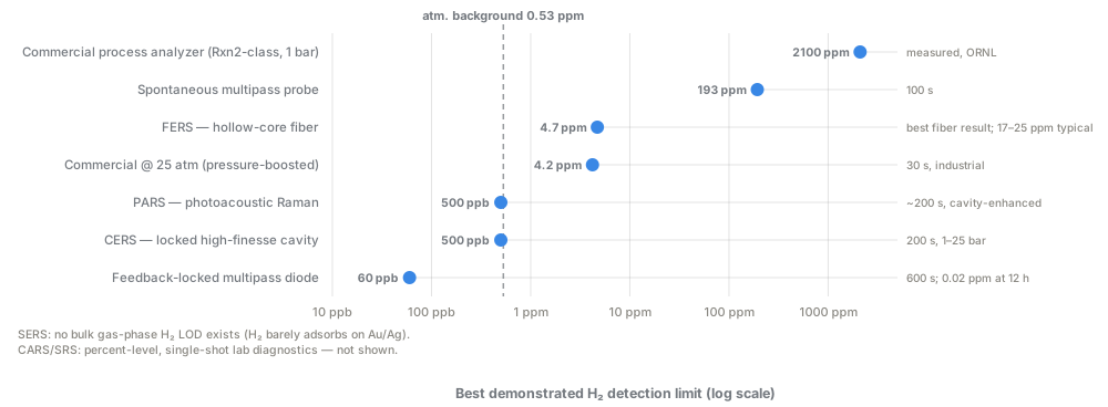
How the enhancement families claw back sensitivity from the spontaneous baseline — the engineering ladder covered in detail on the Enhanced Raman page.

Why pressure and concentration scaling rescue process and mud-gas analysis

Because $n_{H_2}$ (molecules per unit volume), not mole fraction alone, is what enters the photon-budget equation, the same equation says signal scales linearly with total pressure at fixed mole fraction (ideal gas: $n_{tot}=P/k_BT$) and linearly with mole fraction at fixed pressure. Commercial process-gas Raman analyzers — the Endress+Hauser Rxn5, rated to 70 bar/1,000 psi [9], and NETL’s Raman Gas Analyzer, rated to 1,000 psi [13] — routinely see percent-level H₂ in tens-of-bar natural-gas or mud-gas streams.

Compared to the 1 ppm/1 atm scenario above, a 5% H₂ stream at 70 bar has a combined density × mole-fraction product roughly $3.5\times10^{6}$ times larger, turning a ~1–3 photon/s problem into a many-MHz photon-count problem — comfortably inside the 1-second real-time response both NETL and Endress+Hauser quote for their process analyzers [9][13]. This is why every commercial gas-phase Raman analyzer identified in this research is marketed for hydrogen-blending pipelines, turbine fuel gas, and process/syngas composition — high-pressure, percent-level applications — and none is marketed for ambient or soil-gas trace H₂ detection.

The ν⁴ / wavelength trade

Because scattered intensity scales roughly as excitation frequency to the fourth power, moving from a 785 nm to a 532 nm laser for the same H₂ Q-branch shift increases the raw Raman cross section by a factor of ~4.7× using the simple $\nu^4$ rule, or ~7× using the more complete $\nu_L\nu_S^3$ scaling implied by the modern cross-section theory above — both point the same direction.

This is why 532 nm dominates dedicated gas-phase H₂ Raman work (the Endress+Hauser 532 nm option [9], ORNL [2], the NETL Raman Gas Analyzer [13], Fraunhofer IPM’s low-cost hydrogen sensor [14]) even though 785 nm and 1000/1064 nm options exist and are preferred elsewhere in process Raman for lower fluorescence excitation (Metrohm’s 2060 natural-gas analyzer uses 785 nm [15]; tec5’s natural-gas system uses a tunable 785 nm, 35–500 mW laser [8]).

The trade-off is that shorter wavelengths buy signal but also excite more fluorescence in dirty real-world samples (soil organics, drilling mud, window contamination), so vendors split roughly along this line by target market — clean pipeline gas favors 532 nm for signal; messier natural-gas/mud-gas streams favor 785 nm for a cleaner baseline at some sensitivity cost.

Research lineage and current frontiers

Cohen (1972) gave the first careful absolute cross-section measurements for H₂ [6]; Schrötter & Klöckner’s 1979 review chapter [7] became the standard tabulated reference for decades and is still cited in current process-Raman gas literature. The most significant recent advance is Singor, Scarlett, Zammit, Bray & Fursa (2024, Curtin University), whose rigorous, internally consistent set of 9,582 Rayleigh/Raman cross sections, depolarization ratios, and reversal coefficients explicitly reconciles and supersedes older, sometimes-inconsistent literature values [4]. de Groot at NASA (1994) built one of the first fiber-optic backscatter spontaneous-Raman probes aimed specifically at hydrogen leak detection, reporting H₂ “approached the lower limit of detectability” near 2 kPa partial pressure with the detector technology of the day [16].

Among modern applied groups, NETL (Buric, Chorpening, Thapa) runs a DOE-funded program developing a waveguide-enhanced Raman Gas Analyzer explicitly targeted at hydrogen-blend fuel gas composition for turbines, SOFCs, and industrial systems, with an active FY22–FY24 program and a 2025 SPIE paper on real-time hydrogen-blend measurement [13][17]. Andreas Müller’s group (University of South Florida) has done the most work toward field-portable, standoff trace-H₂ Raman sensing via multipass-cavity enhancement (technically cavity-enhanced, not spontaneous — covered properly on the Enhanced Raman page), culminating in 2025 outdoor demonstrations of 63 ppb sensitivity from several meters away, with the authors explicitly flagging “geological prospecting” as a target application [18][19]. ORNL (Peruski et al.) produced the most methodologically transparent, fully quantitative public LOD study for a commercial (non-enhanced) Raman gas analyzer found in this research, explicitly scoped as a nuclear-fuel-cycle feasibility study calling for further work on corrosive streams [2]. A sustained Tomsk/IMCES research program (Petrov, Matrosov, Zaripov, Tanichev) has studied natural-gas Raman analyzer precision and composition cross-effects [20], culminating in a 2025 indirect-helium-via-methane-perturbation quantification method [21]. IS-Instruments, with the University of Southampton’s Optoelectronics Research Centre, has developed hollow-core fiber Raman gas cells aimed at both hydrogen-blending pipelines and fusion-relevant isotopologue analysis [22]. For a broader survey of Raman-based hydrogen detection approaches generally, see Hecht (2020) [23].

The current frontier relevant to Hestia is an engineering problem rather than a physics one: pushing enhancement factors (waveguide/hollow-core, multipass cavities) toward field-ruggedized, lower-cost packages rather than lab optical benches, alongside machine-learning/chemometric spectral deconvolution for dense, overlapping real-gas spectra and cost/size reduction via filter-based, dispersion-free designs.

Variants & subtypes

Within spontaneous, linear, gas-phase Raman, the practical taxonomy is about how the photons are collected rather than a different scattering mechanism (that distinction — spontaneous vs. stimulated vs. coherent multi-wave-mixing — is the boundary to the Enhanced Raman page):

Variant	Distinguishing physics/engineering	Typical LOD regime	Examples
Free-space single-pass dispersive Raman	Laser focused once through an open or windowed gas volume; signal $\propto L\cdot\Delta\Omega$ with $L$ set by focal/cell geometry (mm–cm)	10²–10⁵ ppm	Bench Raman spectrometers, lab demonstrations
Fiber-probe-coupled Raman	Excitation and collection carried by silica fibers to/from a remote probe head; spectrometer, laser, and detector stay at a safe/dry/controlled location	10²–10⁵ ppm (same physics, added deployment flexibility)	Endress+Hauser Rxn-series probes (fiber runs to 500 ft standard) [9]; downhole natural-gas fiber probe with runs to 1,605 m [24]
Multi-reflection (“folded”) probe	Two or more small mirrors around the sample volume recirculate the pump beam and/or re-image scattered light a handful of times, buying a modest (~few×–10×) path-length gain without a true resonant cavity	10¹–10³ ppm	In-situ multi-component probe, LOD 192.9 ppm H₂ with 1.6 W delivered 532 nm [25]
Waveguide/hollow-core-fiber-enhanced Raman	A reflective hollow capillary or hollow-core microstructured fiber confines both pump and scattered light over centimeters-to-meters, multiplying effective $L$ by >10³	1–10² ppm	NETL Raman Gas Analyzer (>1,000× boost) [13][17]; IS-Instruments “Aura” (LOD ~0.04% = 400 ppm) [22] — borders on the enhanced-Raman category
Multipass-cavity / cavity-enhanced Raman (CERS)	An external optical resonator recirculates the pump beam thousands of times (finesse-limited buildup) — a fundamentally different enhancement mechanism from simple folding	ppb–low-ppm	Salter, Chu & Hippler 2012 [26]; Wang et al. 2021 [27]; Singh & Müller 2023 (20–60 ppb) [18]; Arachchige & Muller 2025 (63 ppb, standoff) [19] — fully covered on the Enhanced Raman page
Filter-based / dispersion-free imaging Raman	Replaces the spectrometer+grating with a fixed bandpass filter and a 2-D camera, trading spectral flexibility for size, power, and cost	ppm-range (developmental)	Fraunhofer IPM TransHyDE hydrogen sensor: 532 nm laser, bandpass filter isolating the ~4,150 cm⁻¹ Q-branch, low-cost CMOS camera [14]

A second axis for field planning is rotational (S-branch) vs. vibrational (Q-branch) detection. Most gas-composition instruments read the Q-branch (the clean high-wavenumber window above) for quantification, but a few dedicated H₂ lidar/remote-sensing systems have worked in the rotational window instead, trading closer proximity to the laser line (harder Rayleigh rejection) for larger per-molecule cross sections at low $J$.

Note

A naming trap. Raman-based Distributed Temperature Sensing (DTS), ubiquitous in downhole and pipeline monitoring, is spontaneous Raman scattering physically — but it measures the fiber silica’s own Stokes/anti-Stokes intensity ratio along an ordinary telecom fiber to infer temperature, not the composition of a surrounding gas. It is a completely different application of the same scattering process and is not a gas sensor. “Raman fiber sensing is common downhole” (true, for DTS) does not mean “gas-composition Raman is common downhole” (not yet true at commercial scale).

Performance envelope

All rows describe unenhanced/lightly-folded spontaneous Raman (multipass-cavity/CERS numbers appear only for contrast and are detailed properly on the Enhanced Raman page).

Parameter	Value	Conditions / instrument	Ref
LOD, H₂ (best demonstrated, lab probe)	192.9 ppm	532 nm, 2.5 W laser (1.6 W delivered through fiber), folded 2-mirror probe, 10 s integration	[25]
LOD, H₂ (commercial on-line analyzer)	≈2,100 ppm (≈5% of LEL)	Endress+Hauser Raman Rxn2, 532 nm, up to 15 min exposure / 10 scans, flowing N₂ background	[2]
LOD, H₂ (early fiber-probe prototype, 1994)	≈20,000 ppm (2 kPa in ~100 kPa total)	NASA fiber-optic backscatter probe, pre-CCD-era detector	[16]
Usable range	10² ppm to ~100 vol %	Calibration curves linear 2,100–40,000 ppm ($R^2=0.997$); commercial units calibrated across full 0–100% blends	[2][13]
Response time	1 s (real-time flow-through)	NETL Raman Gas Analyzer, target spec for turbine/SOFC fuel control	[13]
Response time (lab LOD studies)	10 s – 15 min	Trade of integration time vs. sensitivity; longer exposure directly raises SNR	[2][25]
Recovery / cell turnover	Seconds (limited by gas-cell purge/flush, not sensor “recovery” — the scattering itself is instantaneous)	2.3 L/min optimum flow found to maximize SNR in a small flow cell	[2]
Selectivity	High–absolute for major gas identity (unique, resolvable fingerprint per species); not absolute — invisible to monatomic noble gases (He), and dense multi-component natural-gas spectra require chemometric deconvolution	—	[20][21]
Accuracy (process analyzers)	±0.1 vol % per component target spec	NETL RGA design target	[13]
Operating temperature (analyzer body)	−20 to +50 °C	Endress+Hauser Raman Rxn5 enclosure spec	[9]
Operating temperature (probe/sample side, demonstrated)	Ambient to 400 °C (physics still works; commercial probes typically rated lower, ~150 °C)	Deep-sea hydrothermal H₂ Raman study to 400 °C/40 MPa; Endress+Hauser cites 150 °C probe rating	[3][1]
Operating pressure	Up to 70 bar / 1,000 psi	Endress+Hauser Rxn5 pipeline probes; NETL RGA design target	[9][13]
Relative humidity	0–90% non-condensing	Endress+Hauser Rxn5 enclosure spec	[9]
Drift	Low — no consumable, no catalytic surface; managed with laser-power/wavelength reference channels and calibration accessories	Metrohm 2060 has an internal reference channel; Endress+Hauser sells a dedicated Raman Calibration Tool	[15][9]
Power	150 mW (laser only, waveguide-enhanced NETL unit) to <300 W max / <200 W typical (full Rxn5 analyzer incl. laser, spectrometer, TE cooling, electronics)		[13][9]
Physical footprint	Rack-/wall-mount analyzer body (Rxn5: 457×834×254 mm, 61 kg) plus remote fiber probe (fiber runs to 500 ft standard, demonstrated to >1.6 km)		[9][24]
Cost class	~$10,000–$500,000+ general Raman instrument market (handheld to high-performance); dedicated process/gas analyzers skew toward the upper half; exact list prices not publicly disclosed by any vendor found (unverified)		[28]
TRL	9 for the underlying commercial technology as a process/pipeline gas analyzer; 3–4 for any adaptation to trace/soil-gas or downhole formation-gas H₂ detection (no such product identified)	—	—

Figures of merit

The universal figures of merit used to compare any H₂ sensor — sensitivity, LOD, selectivity, response time, drift, and the rest — are defined on the Figures of merit page; concentration units (ppm, vol %, mg/Nm³) follow the conventions on Concentration units. For spontaneous Raman, most of those universal axes are downstream of one physical quantity — the differential Raman scattering cross section — so the table below leads with that and the other modality-specific photon-budget figures before the familiar universal ones.

Figures-of-merit table for this modality (12 rows)

Figure of merit	Symbol / formula	What it means here	Typical value for this technology	How to read it
Differential Raman scattering cross section	$d\sigma/d\Omega$ (cm²·sr⁻¹)	The fixed, physics-set constant giving the probability per molecule per steradian of an inelastic Raman scatter — the modality’s analog of “sensitivity” upstream of any electronics	$(2.70\pm0.43)\times10^{-30}\ \text{cm}^2\text{sr}^{-1}$ at 532 nm, Q-branch [5]; roughly 9–11 orders of magnitude smaller than typical TDLAS/NDIR absorption cross sections ($10^{-19}$–$10^{-21}$ cm²) [4]	This number cannot be improved by better electronics — only by optical enhancement (cavity, waveguide, SERS; see Enhanced Raman) or by raising gas density (next row)
Sensitivity (signal equation)	$\dot N \propto n_{H_2}\cdot(d\sigma/d\Omega)\cdot P\cdot t \;\Rightarrow\; \mathrm{SNR}\propto\sqrt{P\cdot t}$	Photon count is linear in H₂ number density $n_{H_2}$ (i.e., in pressure × mole fraction) and in laser power, but signal-to-noise only improves with the square root of power times integration time	Scaling a 5% H₂ stream from 1 atm to 70 bar raises the density×mole-fraction product by ≈3.5×10⁶× relative to a 1 ppm/1 atm scenario (see the pressure/concentration scaling discussion above)	Doubling laser power or integration time buys only ~1.4× SNR; this square-root scaling is why trace-level LOD gains require optical enhancement rather than a bigger laser
Photon count rate / photon budget	$\dot N \approx \Phi_L\, n_{H_2}\,(d\sigma/d\Omega)\,\Delta\Omega\, L$	The absolute rate of Raman photons reaching the detector — the real “signal” the instrument has to work with before spectrometer/CCD losses	~1–3 photons/s (idealized) for 1 ppm H₂, 1 atm, 100 mW @ 532 nm, NA 0.22, $L$ = 1 cm (see the explicit photon-budget arithmetic above [5][8][9]); scales to a many-MHz count rate at 5% H₂/70 bar	This number separates “usable today” (percent-level process gas) from “not usable” (ppm-level soil gas); the other rows in this table follow from it
Limit of detection (LOD)	Defined on the Figures of merit page; no single $k$/integration-time convention is common across the sources below	Smallest H₂ concentration reliably told apart from background, at a stated integration time; report it together with that time	192.9 ppm, folded 2-mirror probe, 1.6 W delivered, 10 s integration [25]; ≈2,100 ppm, commercial on-line analyzer, up to 15 min exposure / 10 scans [2]	The >10× gap between these two numbers is driven partly by integration time and partly by fluorescence (below), not purely by hardware quality; the relevant figure is the LOD at a stated integration time $t$
Selectivity / cross-sensitivity	$1/\max_j(K_{ij})$ (see Figures of merit)	Each Raman-active gas occupies a distinct, resolvable line, so H₂’s cross-sensitivity to co-evolved gases is close to zero in principle	High–near-absolute among Raman-active species: H₂ (354/587/4,155 cm⁻¹) fully resolved from CH₄ (≈2,917), CO₂ (1,285/1,388), N₂ (≈2,330), H₂S (≈2,611 cm⁻¹) [2]; zero selectivity for He — monatomic, no Raman activity at all	The one hard blind spot is helium, an important co-tracer gas; an indirect CH₄-perturbation workaround exists but is single-group and unreplicated [21]
Spectral resolution	$\Delta\tilde\nu$ (cm⁻¹)	How finely the spectrometer resolves adjacent lines — needed to separate the Q₁(0)–Q₁(3) comb (4,126–4,161 cm⁻¹) and to confirm species identity against neighboring gases	5 cm⁻¹ (Endress+Hauser Rxn5/Rxn2 instrument resolution) [9]	Coarser than ideal for fully separating the Q-branch comb from itself, but adequate because H₂’s windows are uncrowded relative to other gases (see Mechanism & physics above) — resolution demand is dominated by inter-species discrimination, not intra-H₂ line splitting
Fluorescence rejection	No standardized numeric figure; qualitatively, fluorescence baseline height vs. Raman peak height	Broadband fluorescence from soil organics, dust, mud, or cell-window contamination competing with the already-weak Raman signal — the dominant real-world noise floor, not shot noise	ORNL explicitly reports “a significant fluorescence baseline” growing with exposure time/scan count as the limiting factor behind the measured 2,100 ppm LOD [2], versus the ~1–3 photon/s idealized photon-budget estimate above that ignores it	The gap between the idealized ~1 ppm-class estimate and the measured 2,100 ppm LOD is explained almost entirely by fluorescence, not cross-section physics — the practical reason 532 nm (more signal, more fluorescence) and 785 nm (less signal, cleaner baseline) vendors split by target market
Response / recovery time	—	How fast a reading tracks a real concentration change, and how fast it returns to baseline once gas clears	1 s real-time flow-through target (NETL) [13]; 10 s–15 min for lab LOD studies, trading integration time for sensitivity [2][25]; recovery limited by gas-cell purge/flush (seconds), not scattering kinetics (instantaneous) [2]	Directly coupled to the Sensitivity row above — faster response always costs LOD at fixed laser power, and vice versa
Dynamic / linear range	$N_{\text{decades}}=\log_{10}(C_{\max}/C_{\min})$	Full span of usable concentration, and the (unusually large) sub-span where photon count is genuinely linear in concentration	~10² ppm to ~100 vol % usable; calibration linear 2,100–40,000 ppm, $R^2=0.997$ [2]; full 0–100% blends calibrated commercially [13]	Because signal is literally a photon count, linearity holds across nearly the entire usable range — unlike the intrinsically log-linear response of MOX/FET sensors (see Figures of merit)
Drift / stability	—	Baseline and sensitivity creep over time	Low — no consumable, no catalytic surface to poison; the main long-term risk is laser power/wavelength drift over lamp life	Managed with reference channels (Metrohm 2060’s internal reference) or a dedicated calibration accessory (Endress+Hauser Raman Calibration Tool), not a fixed one-time factory curve [15][9]
Power	—	Electrical draw, which trades directly against LOD via the Sensitivity row above	150 mW laser-only (NETL waveguide-enhanced unit) to <300 W max / <200 W typical for a full analyzer (laser + spectrometer + TE cooling + electronics) [13][9]	A brighter laser buys LOD headroom at the cost of power budget and laser-safety overhead (Class 3B/4 lasers, ATEX/IECEx-rated enclosures) [9]
Operating envelope	$C_{\text{reported}} = C_{\text{raw}}\cdot f_T(T)\cdot f_{RH}(RH)\cdot f_P(P)$ (see Figures of merit)	Where the stated accuracy actually holds, distinct from where the instrument merely survives	Analyzer body: −20 to +50 °C, 0–90% RH non-condensing, up to 70 bar/1,000 psi [9]; probe/sample-side physics demonstrated to 400 °C/40 MPa, though commercial probes are typically rated to ~150 °C [3][1]	The Raman shift is nearly temperature-independent, but signal strength is not — density (∝1/T at fixed pressure) and Q-branch broadening both demand a temperature/pressure-corrected calibration for downhole use, not a single lab curve [3]

What dominates. Two figures of merit decide whether spontaneous Raman is usable for a geologic-H₂ job: the fixed differential cross section ($d\sigma/d\Omega\sim10^{-30}$ cm²/sr) sets an absolute photon budget no amount of downstream engineering can change, and the resulting $\mathrm{SNR}\propto\sqrt{P\cdot t}$ relation then forces a hard three-way trade between LOD, response time, and laser power — halving LOD costs 4× the integration time or 4× the optical power, not a modest upgrade. Because the cross section itself is fixed, the lever operators actually pull is gas density: raising pressure from 1 atm to tens of bar buys orders of magnitude of signal for free, which is exactly why spontaneous Raman is mature for percent-level pipeline/process gas [9][13] but stalls at hundreds-to-thousands of ppm at atmospheric-pressure, soil-gas-relevant concentrations [2][25]. Selectivity and drift, by contrast, are essentially non-issues here (Raman’s main strength is exactly the multi-gas fingerprint, and there is no catalytic surface to poison); the real second-order threat is fluorescence, which in practice — not shot noise — is what separates the idealized ~1 ppm photon-budget estimate from the ~2,100 ppm measured field LOD [2].

Environmental covariance & cross-sensitivity

Temperature. The Raman shift of a given transition is a molecular property and is nearly temperature-independent to first order, but gas density at fixed pressure scales as $1/T$, so signal strength itself drifts with temperature unless density-normalized. At elevated temperature and pressure, H₂’s vibrational Q-branch shows measurable wavenumber shift and band broadening — a dedicated study to 400 °C and 40 MPa (conditions relevant to deep hydrothermal or downhole fluids) found “strong density and temperature dependences of the wavenumber and bandwidth” of the gaseous H₂ vibrational band [3] — meaning a downhole deployment needs either a temperature/pressure-corrected calibration or in-situ reference lines, not a single lab calibration curve. Elevated temperature at the detector also raises CCD dark current unless thermoelectrically cooled, and raises the thermal/fluorescence background from optics and sample-cell windows.

Pressure/density. This is the dominant, and favorable, covariate: signal scales linearly with total number density, which every commercial process analyzer exploits deliberately. The flip side is that quantification requires either an internal pressure-corrected calibration or an internal reference line — e.g., using N₂’s own Raman peak as an internal density standard, as ORNL implicitly did by working in an N₂ background [2].

Humidity / water vapor. Water’s O–H stretch bands sit at 3,000–3,700 cm⁻¹ (scattered at ≈633–662 nm for a 532 nm pump), well clear of both the H₂ rotational window (300–1,100 cm⁻¹; ≈541–565 nm) and the H₂ Q-branch (4,100–4,200 cm⁻¹; ≈680–685 nm) — ORNL explicitly checked and confirmed no direct spectral overlap [2]. This is a genuine advantage over techniques that are humidity-cross-sensitive at the sensing-element level (electrochemical cells, MOx). However, humidity is a first-order confound for the geology, not the photon budget: in the one directly comparable soil-gas field study found, hydrogen flux was highest when relative humidity was below 65% and fell as RH rose toward 74%, a much stronger correlate than temperature ($r^2=0.13$) or pressure ($r^2=0.11$) [11]. In other words, Raman itself is insensitive to ambient RH, but interpreting an H₂ Raman reading as a subsurface signal requires tracking RH as a transport/emission covariate.

Co-evolved gases (CH₄, CO₂, N₂, CO, H₂S). This is Raman’s main strength: one 532 or 785 nm laser illuminates the sample once, and the detector simultaneously records every Raman-active species’ unique fingerprint — H₂ (354/587/4,155 cm⁻¹), N₂ (≈2,330 cm⁻¹, directly confirmed in ORNL’s own spectra [2]), CH₄ (≈2,917 cm⁻¹), CO₂ (Fermi dyad at 1,285/1,388 cm⁻¹), CO (≈2,143 cm⁻¹), and H₂S (≈2,611 cm⁻¹) all appear as distinct, non-overlapping peaks in a single spectrum. Mud-logging and natural-gas literature repeatedly makes exactly this point: Raman provides excellent chemical selectivity that allows identification of almost all hydrocarbon and non-hydrocarbon gases except noble gases. The practical caveat is that dense real gas mixtures cause line broadening and small shifts in each other’s bands, which is why real natural-gas/mud-gas Raman analyzers lean on chemometric or neural-network deconvolution rather than simple peak-height lookup once more than 2–3 species are present at comparable concentration.

Helium — an explicit, important gap. Helium is monatomic: it has no bonds, therefore no vibrational or rotational modes, and therefore produces no Raman shift at all — it is invisible to Raman spectroscopy by the same physics that makes noble gases IR-silent. Because He is a diagnostically important co-migrating tracer gas in natural-hydrogen systems, this is a serious limitation for using Raman alone as a complete gas-fingerprinting tool. Recent work (Tanichev & Petrov, 2025) developed an indirect workaround: He’s presence perturbs the pressure-shift and pressure-broadening of the CH₄ ν₁ band, allowing He content to be inferred (not directly measured) with roughly 1 mol% standard uncertainty at 50 bar, improvable to ~0.01 mol% with a high-resolution spectrometer — explicitly framed by the authors as “a valuable addition to comprehensive natural gas analysis rather than a replacement for dedicated helium detectors” [21]. For Hestia’s purposes, any Raman-based multi-gas station still needs a separate He channel (mass spectrometry, or a dedicated He leak-detector-style sensor) if He is a target tracer.

Fluorescence and ambient light. This is the largest practical failure mode. Real soil/mud-gas samples carry trace organics, dust, and mineral particulates; visible-wavelength (532 nm) excitation readily drives broadband fluorescence that can swamp the already-weak Raman signal — ORNL explicitly notes their instrument’s high-energy excitation source produces “a significant fluorescence baseline” with increased scan number/exposure time [2]. This is the standard 532-vs-785/1064 nm engineering trade already discussed above. Outdoor daylight or artificial ambient light is a second, unrelated background source that any open-path or standoff Raman system must reject via narrow bandpass filtering, enclosed sample cells, or gated/pulsed detection — the portable standoff hydrogen Raman analyzer explicitly tested laboratory, atrium, and outdoor conditions to validate this [19][22].

“Poisoning” and fouling. Raman has no catalytic surface, membrane, or electrode to poison — a genuine advantage over pellistor/electrochemical/MOx sensors, and the explicit motivation for ORNL’s interest in Raman for corrosive, O₂-free nuclear-fuel-cycle off-gas streams where “many [other] techniques are not compatible with corrosive or O₂-free gas streams or cannot be used in on-line monitoring” [2]. The Raman analog of poisoning is optical fouling: soot, oil mist, scale, or condensation on cell windows or fiber facets attenuates both excitation and collection throughput over time and must be managed by purge gas, window maintenance, or probe design.

Laser safety / systems overhead. Not a gas cross-sensitivity but a deployment-relevant failure mode: these are Class 3B/4 laser systems. Field/process units require ATEX/IECEx/CSA-rated enclosures and interlocked fiber connectors for hazardous-area use (Endress+Hauser Rxn5 carries ATEX, CSA, IECEx, UKCA, JPEx, KCs certification) [9] — a genuine cost, complexity, and maintenance overhead relative to a simple electrochemical cell.

Use for geologic H₂

Field verdict

Unenhanced spontaneous Raman cannot see soil-gas or atmospheric-background H₂. The best directly demonstrated LOD in the literature for an unenhanced or lightly-folded spontaneous system is ~190 ppm [25]; a real commercial on-line analyzer measured ~2,100 ppm [2]. Both sit far above the 0.53 ppm atmospheric background and, for the ~190 ppm case, above much of the 1–1,000 ppm soil-gas anomaly range reported in a directly comparable field comparison study [11]. This is a consequence of the ~10⁻³⁰ cm²/sr cross section (above), not something better electronics can fix, and the fix (cavity enhancement, hollow-core/waveguide confinement) is a different technology covered on the Enhanced Raman page. Where spontaneous Raman genuinely excels today is percent-level composition of a flowing, pressurized gas stream: pipeline blending, turbine fuel gas, and process/syngas monitoring are mature, off-the-shelf commercial applications, not a research project.

Soil-gas surveys. Not viable with unenhanced spontaneous Raman, given the numbers above. A field campaign targeting the 1–1,000 ppm anomaly window (and the sub-ppm background needed to establish a baseline) needs either an enhanced-Raman variant (see Enhanced Raman) or a different modality entirely. Where spontaneous Raman can add value in a soil-gas context is opportunistically, at a confirmed strong seep or vent where concentrations already reach the percent level — there it offers a genuine single-instrument, single-laser compositional fingerprint (H₂ + CH₄ + CO₂ + N₂ + H₂S simultaneously) without the cross-sensitivity problems of electrochemical or MOx sensors, useful for characterizing a known active site rather than discovering one. A broader review of soil-gas survey design for natural hydrogen seepage frames the same methodology landscape and anomaly window [29].

Continuous monitoring stations. The one directly comparable field deployment found in this research (Harvey, Perth Basin) used electrochemical (GA5000, iBrid Mx6) and IR (WHALI autonomous unit) sensors for continuous soil-gas tracking, not Raman [11] — consistent with the sensitivity gap above. A mains-powered, fixed continuous-monitoring station could host an enhanced-Raman instrument (multipass/CERS units have reached 20–63 ppb in research settings [18][19]), but a plain spontaneous-Raman station would need to be sited at, or downstream of, a known strong seep to have any chance of seeing a real signal continuously.

Downhole deployment. This is the most promising near-term fit, and it matches a strong architectural preference for no downhole electronics almost exactly: only a passive optical fiber and probe optics need go downhole; the laser, spectrometer, and detector stay at the surface. There is direct precedent — a downhole natural-gas Raman composition system used a 785 nm spectrometer coupled through fiber runs up to 1,605 m to a wellbore probe, successfully derived gas molar composition via regression/neural-network calibration, and separately detected H₂S down to 1–3 mg/Nm³ [24]. Endress+Hauser’s fiber probes are rated to 70 bar/150 °C today [9][1], and the underlying photon-budget argument above means this approach is genuinely strong for percent-level composition of a flowing or sampled gas stream, but it inherits the same trace-level sensitivity gap as soil-gas surveys if the goal is detecting low-ppm formation-gas H₂ in equilibrium at depth rather than measuring an already-flowing, concentrated show. An SPE 2025 review of advanced mud-gas logging for H₂ exploration explicitly frames current best practice around GC-MS calibrated below 5 ppm and lists cavity-enhanced Raman spectroscopy only as an emerging, not-yet-standard improvement path — i.e., industry’s own assessment agrees spontaneous Raman is not there yet for trace mud-gas H₂ [30].

Process/pipeline/mud-gas composition (adjacent infrastructure, not exploration). This is where spontaneous Raman is already a mature, commercially deployed, and genuinely excellent solution — percent-level H₂ in high-pressure natural gas blending, turbine fuel gas, and syngas streams [13][17][1][9][8][15][20]. If Hestia’s downstream operations ever involve confirming H₂ content in produced or blended gas at pipeline-relevant pressures and concentrations, this is a proven, off-the-shelf technology class.

Helium blindness, again. In the field-deployment context: if a survey design leans on He as a co-tracer (a common practice in natural-H₂ exploration), a pure Raman station cannot provide that channel directly and needs a companion instrument.

Vendors & products

For a vendor-neutral primer on process Raman analyzer principles generally, see Swagelok’s technical overview [31].

Vendor	Product / line	Laser	Key specs	TRL / market status	Price class	Source
Endress+Hauser (ex-Kaiser Optical Systems)	Raman Rxn5 (SKU KRXN5C, predecessor KRXN5B)	532 nm	150–3,425 cm⁻¹ range (≈536–651 nm scattered), 5 cm⁻¹ resolution; up to 4 channels; <300 W max/<200 W typical; −20 to +50 °C; 0–90% RH; IP56; ATEX/CSA/IECEx/UKCA/JPEx/KCs; fiber probes to 500 ft standard, rated to 70 bar/150 °C	Commercial, mature (TRL 9)	High (list price not public; general Raman market $10k–$500k+)	[9]
Endress+Hauser	Raman Rxn2 (benchtop/mobile-cart)	532/785/1000 nm options	150–4,350 cm⁻¹ (≈536–692 nm scattered, 532 nm base), 5 cm⁻¹ res.; 15–30 °C operating range	Commercial, mature	High	[2][9]
Endress+Hauser / Kaiser Optical	RamanRXn1	NIR (“Invictus” laser)	HoloPlex grating for single-shot full-spectrum acquisition; gas-phase probe accessory available	Commercial, mature	High	[32]
Metrohm (ex-B&W Tek)	2060 Raman Analyzer	785 nm	Continuous inline process monitoring; up to 5 sampling streams; integrated reference channel for calibration	Commercial	High	[15]
tec5 (tec5USA)	Raman Spectrometer for natural gas	785 nm, tunable 35–500 mW	1024×58 CCD, VPH transmission gratings, 300–3,100 cm⁻¹ (≈804–1,038 nm scattered at 785 nm); Hellma Multipass Probe / tecRaman probe options	Commercial	Mid–High	[8]
IS-Instruments (with Univ. Southampton ORC, Jacobs)	Aura gas Raman analyzer	Not disclosed	Hollow-core micro-structured optical fiber sample cell; LOD “as low as 0.04%” (~400 ppm); resolves H₂/D₂/HD isotopologues; applications in H₂ pipeline blending, industrial emissions, fusion (tritium)	Commercial/early-commercial	Not disclosed	[22]
NETL / DOE (Chorpening, Thapa, Buric)	Raman Gas Analyzer (RGA), compact rack-mount prototype	532 nm, 150 mW	Reflective hollow waveguide gives >1,000× signal boost; 1 s measurement target; 0.1 vol % accuracy target; up to 1,000 psi; US Patent 8,674,306	Prototype, TRL ~5–6, tech-transfer stage	Not commercial yet	[13][17][33]
Fraunhofer IPM	Low-cost filter-based H₂ Raman sensor (TransHyDE project)	532 nm	Bandpass-filtered detection of the ~4,150 cm⁻¹ (≈683 nm scattered) Q-branch onto a low-cost CMOS camera; portable/mobile testing-station form factor	Prototype/pre-commercial	Low (explicit design goal)	[14]
Academic — Andreas Müller group (Univ. South Florida)	Portable multipass-cavity H₂ Raman analyzer	Multimode blue laser diode	20–60 ppb LOD (research-grade, technically cavity-enhanced — see Enhanced Raman page); standoff detection of 63 ppb excess H₂ from several meters outdoors	Research prototype	Not commercial	[18][19]
Academic — M. Hippler group	CERS with optical-feedback cw diode lasers	635 nm diode	ppm-by-volume noise-equivalent LOD at 10 mW; foundational CERS design later extended to natural-gas and hydrogen-fuel-cell impurity work	Research	Not commercial	[26]
ORNL (Peruski et al.)	In-house on-line H₂ Raman test rig (uses a Kaiser Rxn2 as the spectrometer)	532 nm	Demonstrated 2,100 ppm LOD for flowing H₂ in N₂; developed for nuclear-fuel-cycle corrosive off-gas monitoring, not a commercial product	Applied research, TRL ~4	N/A	[2]
Tomsk group (Petrov, Matrosov, Zaripov, Tanichev)	Raman natural-gas analyzer studies (composition-precision effects, He-via-CH₄ method)	Not disclosed	Demonstrated indirect He quantification via CH₄ ν₁ perturbation (~1 mol% std., ~0.01 mol% w/ high-res spectrometer at 50 bar)	Research	N/A	[20][21]

Open questions

1. No published soil-gas or ambient trace-H₂ field trial of unenhanced spontaneous Raman was found. Everything quantitative on trace-level performance in this page comes from process-gas/lab studies (ORNL, multi-reflection probe demonstrations) or from enhanced variants that belong on the Enhanced Raman page. If Hestia or anyone else runs a field comparison, it would be a genuinely novel data point.
2. Get an authoritative absolute cross-section value directly from the Singor et al. 2024 dataset [4] rather than relying on the independently sourced lidar value [5] — the two should agree, but a primary-source number would tighten the cross-section discussion.
3. Confirm the “H₂ ≈ 2.2× N₂” cross-section ratio at 514.5 nm [7] directly from the Schrötter & Klöckner full text rather than a secondary citation.
4. Investigate whether any vendor’s fiber-probe Raman system has actually been run at true downhole reservoir pressure/temperature (not just the 70 bar/150 °C probe rating). The downhole natural-gas fiber-probe paper [24] is the closest precedent found, but its exact well depth/P/T conditions warrant direct follow-up.
5. He-workaround validation. The indirect He-via-CH₄ method [21] is new and single-group; treat it as unconfirmed by independent replication before relying on it for tracer-gas work.
6. Confirm current commercial pricing for Endress+Hauser Rxn5/Rxn2, Metrohm 2060, and IS-Instruments Aura — none publish list prices; a real quote would sharpen the cost-class row materially.
7. Chase the mud-gas-logging industry consensus forward. The SPE 2025 review [30] frames CERS as “emerging, not current” for trace mud-gas H₂ — worth periodically re-checking whether that assessment has shifted as enhanced-Raman field hardware matures.

Related pages

• Why H₂ is a hard sensing target
• Enhanced Raman (CERS, fiber, SERS & coherent Raman) — the ppb-to-low-ppm-capable sister techniques referenced throughout this page
• IR absorption and proxies
• UV/EUV and fluorescence
• Fiber-optic sensors — the leading passive, no-downhole-electronics alternative for the same wellbore niche
• Electrochemical cells — the incumbent soil-gas survey tool Raman cannot yet match on sensitivity
• Plasmonic metamaterials — SERS-adjacent field-enhancement physics
• Geologic context for H₂ exploration

References

Full reference list (0 entries)

[1] Endress+Hauser. “How to measure hydrogen in natural gas with Raman spectroscopy.” https://endressprocessautomation.com/how-to-measure-hydrogen-in-natural-gas-with-raman-spectroscopy/

[2] Peruski, K. M.; Vestal, B. K.; Vick, M.; Cobble, C.; Johnson, K. R.; McFarlane, J. “On-line Measurement of Hydrogen Gas using Raman Spectroscopy for Process Gas Systems.” ORNL/TM-2023/2949, Oak Ridge National Laboratory, July 2023. https://info.ornl.gov/sites/publications/Files/Pub195932.pdf; https://www.osti.gov/biblio/1988350

[3] Li, L.; Zhang, X.; Luan, Z.; Du, Z.; Xi, S.; Wang, B.; Cao, L.; Lian, C.; Yan, J. “Raman vibrational spectral characteristics and quantitative analysis of H2 up to 400 °C and 40 MPa.” J. Raman Spectrosc. 49(10), 1722–1731 (2018). DOI: 10.1002/jrs.5420.

[4] Singor, A. J. C.; Scarlett, L. H.; Zammit, M. C.; Bray, I.; Fursa, D. V. “Rovibrationally resolved Rayleigh and Raman scattering cross sections for molecular hydrogen.” J. Chem. Phys. 161, 244304 (2024). DOI: 10.1063/5.0235703. https://pubs.aip.org/aip/jcp/article/161/24/244304/3328533/ ; PubMed: https://pubmed.ncbi.nlm.nih.gov/39727281/

[5] Privalov, V. E.; Shemanin, V. G. “Lidar Measurement of the Raman Differential Cross Section by Hydrogen Molecules.” Optical Memory and Neural Networks 32, 34–38 (2023). https://link.springer.com/article/10.3103/S1060992X23010034

[6] Cohen, E. R. et al. “Absolute Raman Scattering Cross-Section of Molecular Hydrogen.” Astrophysical Journal 178, 551 (1972). https://ui.adsabs.harvard.edu/abs/1972ApJ…178..551C

[7] Schrötter, H. W.; Klöckner, H. W. “Raman Scattering Cross Sections in Gases and Liquids.” In Raman Spectroscopy of Gases and Liquids (Topics in Current Physics, vol. 11), ed. A. Weber, Springer, Berlin/Heidelberg, 1979, pp. 123–166. https://link.springer.com/chapter/10.1007/978-3-642-81279-8_4

[8] AZoM / tec5USA. “Using In-Line Raman Spectroscopy for Natural Gas Monitoring.” https://www.azom.com/article.aspx?ArticleID=20110

[9] Endress+Hauser. “Raman Rxn5 process analyzer” and “Raman Rxn2 analyzer” product/technical-information pages. https://www.us.endress.com/en/field-instruments-overview/optical-analysis-product-overview/raman-rxn5-analyzer; https://www.endress.com/en/field-instruments-overview/optical-analysis-product-overview/raman-rxn2-analyzer

[10] Ibsen Photonics. “The effect of cooling CCD detectors for spectroscopy.” https://ibsen.com/resources/detector-resources/the-effect-of-cooling-ccd-detectors-for-spectroscopy/

[11] Davies, K.; Haines, P. W.; Thomas, C.; Normore, L. “Natural hydrogen soil gas emissions near Harvey, Perth Basin: a comparative study of survey methods.” Science and Technology for Energy Transition 80, 46 (2025). DOI: 10.2516/stet/2025026. https://www.stet-review.org/articles/stet/full_html/2025/01/stet20250031/stet20250031.html

[12] Edmund Optics. “532 nm, 25 mm Dia., OD 6.0 Blocking Notch Filter” (representative notch-filter spec). https://www.edmundoptics.com/p/532nm-25mm-dia-od-6-blocking-notch-filter/28612/

[13] Chorpening, B.; Thapa, J.; Buric, M. “Raman Gas Analyzer for Real-time Gas Composition Monitoring.” DOE Hydrogen Program 2023 Annual Merit Review and Peer Evaluation Meeting, Project ID FE018, National Energy Technology Laboratory, 2023. https://www.hydrogen.energy.gov/docs/hydrogenprogramlibraries/pdfs/review23/fe018_chorpening_2023_p-pdf.pdf

[14] Fraunhofer IPM. “Raman spectroscopy on gases”; “Sensors for safe use of hydrogen” (TransHyDE project hydrogen Raman sensor). https://www.ipm.fraunhofer.de/en/bu/gas-and-process-technology/applications/environment/raman-spectroscopy-on-gases.html; https://www.ipm.fraunhofer.de/en/press-publications/press-releases/sensors-for-safe-use-of-hydrogen.html

[15] Metrohm. “2060 Raman Analyzer” product page. https://www.metrohm.com/en/products/process-analyzers/2060-raman-analyzer.html

[16] de Groot, W. A. (NYMA, Inc., for NASA Lewis Research Center). “The Use of Spontaneous Raman Scattering for Hydrogen Leak Detection.” AIAA-1994-2983; NASA-CR-195373; NASA Technical Reports Server 19950004589. https://ntrs.nasa.gov/citations/19950004589

[17] Thapa, J.; Buric, M. P.; Chorpening, B. T. “Real-time hydrogen gas blend composition measurement with waveguide-enhanced Raman gas analyzer.” Proc. SPIE 13467, Optical Waveguide and Laser Sensors IV, 134670G (2025). DOI: 10.1117/12.3053587. https://www.spiedigitallibrary.org/conference-proceedings-of-spie/13467/134670G/

[18] Singh, J.; Müller, A. “High-Precision Trace Hydrogen Sensing by Multipass Raman Scattering.” Sensors 23(11), 5171 (2023). DOI: 10.3390/s23115171. https://pmc.ncbi.nlm.nih.gov/articles/PMC10255963/

[19] Arachchige, C. M.; Muller, A. “Portable Raman hydrogen concentration mapping with parts-per-billion sensitivity.” Applied Optics 64(13), 3646–3654 (2025). DOI: 10.1364/AO.558965. https://opg.optica.org/ao/abstract.cfm?uri=ao-64-13-3646

[20] Petrov, D. V.; Matrosov, I. I.; Zaripov, A. R.; Tanichev, A. S. “Raman Natural Gas Analyzer: Effects of Composition on Measurement Precision.” Sensors 22(9), 3492 (2022). DOI: 10.3390/s22093492. https://pmc.ncbi.nlm.nih.gov/articles/PMC9099776/

[21] Tanichev, A. S.; Petrov, D. V. “Helium Detection in Natural Gas Using Raman Spectroscopy.” Applied Spectroscopy 79(5), 784–796 (2025). DOI: 10.1177/00037028241282669. https://pubmed.ncbi.nlm.nih.gov/39380533/

[22] IS-Instruments. “Aura — characterising gases using Raman” (hollow-core micro-structured optical fibre gas Raman analyzer). https://is-instruments.com/characterising-gases-using-hollow-core-micro-structured-optical-fibre/

[23] Hecht, E. S. “Hydrogen detection via Raman scattering.” SAND2020-11172PE, Sandia National Laboratories, October 2020. https://www.osti.gov/biblio/1826452

[24] Dąbrowski, A.; Kuczyński, S.; Barbacki, J.; Włodek, T.; Smulski, R.; Nagy, S. “Downhole measurements and determination of natural gas composition using Raman spectroscopy.” Journal of Natural Gas Science and Engineering 65, 25–31 (2019). https://www.sciencedirect.com/science/article/abs/pii/S1875510019300411

[25] Guo, J.; Luo, Z.; Liu, Q.; Yang, D.; Dong, H.; Huang, S.; Kong, A.; Wu, L. “High-Sensitivity Raman Gas Probe for In Situ Multi-Component Gas Detection.” Sensors 21(10), 3539 (2021). DOI: 10.3390/s21103539. https://pmc.ncbi.nlm.nih.gov/articles/PMC8160845/

[26] Salter, R.; Chu, J.; Hippler, M. “Cavity-enhanced Raman spectroscopy with optical feedback cw diode lasers for gas phase analysis and spectroscopy.” Analyst 137(20), 4669–4676 (2012). https://pubs.rsc.org/en/content/articlelanding/2012/an/c2an35722d

[27] Wang, P.; Chen, W.; Wang, J.; Zhou, F.; Hu, J.; Zhang, Z.; Wan, F. “Hazardous Gas Detection by Cavity-Enhanced Raman Spectroscopy for Environmental Safety Monitoring.” Anal. Chem. 93(46), 15474–15481 (2021). DOI: 10.1021/acs.analchem.1c03499.

[28] Excedr. “Raman Spectroscopy Instrument Pricing: A Comprehensive Guide.” https://www.excedr.com/blog/raman-spectroscopy-instrument-pricing-guide

[29] “Exploring Natural Hydrogen Hotspots: A Review and Soil-Gas Survey Design for Identifying Seepage.” Geoenergy (Geological Society, London), 2023. https://www.earthdoc.org/content/journals/10.1144/geoenergy2023-014

[30] “Advanced Mud Gas Logging Techniques for Hydrogen Exploration.” SPE Middle East Oil and Gas Show and Conference, OnePetro D011S018R002 (2025). https://onepetro.org/SPEMEOS/proceedings-abstract/25MEOS/25MEOS/D011S018R002/790177

[31] Swagelok. “Know Your Process Analyzers: Raman Analyzers.” https://www.swagelok.com/en/blog/process-analyzers-raman-analyzers-what-to-know

[32] Eastern Controls, Inc. “Kaiser Optical RamanRXn1 Analyzer.” https://www.easterncontrols.com/product-focus/2017/06/12/kaiser-optical-ramanrxn1-analyzer/

[33] National Energy Technology Laboratory. “Raman Gas Analyzer” R&D Fact Sheet R-D106 (June 2022) and “Raman Gas Analyzer for Natural Gas and Syngas Applications.” https://netl.doe.gov/sites/default/files/rdfactsheet/Fact%20Sheet%20R-D106,%20June%202022,%20Raman%20Gas%20Analyzer.pdf (link dead) ; https://netl.doe.gov/node/14324