Environmental covariance & signal interpretation

Summary

A field H2 reading is distorted twice before it reaches a screen. First, the sensor behaves differently with the weather: cold mornings, humid afternoons, and the sampling pump switching on nudge a reading by amounts that rival the target signal. Second, the actual amount of H2 escaping the ground is itself weather-controlled, independent of geology: rain caps a seep, a falling barometer pumps gas out faster, and the soil bacteria that consume H2 speed up or slow down with temperature and moisture. A passing weather front can make a real seep look bigger, smaller, or manufacture one where none exists, through several distinct physical channels that arrive in the same reading, often pointing the same way at once.

This page separates those effects: the physics, the measured error sizes per sensor family, and the monitoring and statistical practices that tell a genuine geologic pulse from drift, noise, and last week’s rain.

The numbers to remember

Single-covariate regressions of field H2 against temperature or barometric pressure alone explain only ~11–13% of the variance in published data; multivariate/harmonic correction is not optional. Layer-1 sensor artifacts and Layer-2 signal swings routinely sit at the same order of magnitude as the anomaly: soil moisture alone can suppress a genuine reading ~10×, and 1% co-evolved helium can bias a thermal-conductivity channel by ~+7,700 ppm H2-equivalent. No raw reading is interpretable without simultaneous logging of soil temperature, moisture, barometric pressure (and its rate of change), and gas-line relative humidity.

How it works

Two confounding layers. Every reading is the output of a chain with two distinct sources of environmental sensitivity stacked on the quantity of interest:

$$R_{\text{measured}} = g\Big(C_{H_2}^{\text{geologic}}(z,t) + C_{H_2}^{\text{biogenic}}(z,t) - C_{H_2}^{\text{microbial sink}}(z,t)\Big)\Big|_{T,\,RH,\,P,\,\text{matrix}}$$

Layer 1 (sensor covariance) is the dependence of the transfer function $g(\cdot)$ itself on temperature, humidity, pressure, and co-occurring gases. A first-order expansion makes it explicit:

$$R \approx R_0 + S_0\,\Delta C_{H_2} + \frac{\partial R}{\partial T}\Delta T + \frac{\partial R}{\partial RH}\Delta RH + \frac{\partial R}{\partial P}\Delta P + \sum_i \kappa_i \Delta C_i$$

where $S_0$ is nominal sensitivity and $\kappa_i$ are cross-sensitivity coefficients to interferent $i$ (CO, CH4, CO2, H2S, He). For every family here, the covariate partial derivatives are the same order as $S_0\,\Delta C_{H_2}$ or larger at exploration concentrations. The working figure of merit is the signal-to-covariate ratio, $\mathrm{SCR} = \Delta C_{H_2}^{\text{true}} / \Delta C_{H_2}^{\text{covariate-equivalent}}$; every quantitative table below estimates one term in that denominator.

Layer 2 (signal covariance) is that the geologic, biogenic, and microbial-sink terms are themselves functions of the same environmental variables corrupting the sensor in Layer 1, so the confound is structurally correlated with the sensor artifact rather than additive noise. A temperature rise can accelerate microbial uptake or drive advective outgassing while simultaneously shifting an electrochemical cell’s zero current and a MOX baseline, in the same record, at the same time, in directions not separable from one spot reading.

Governing transport equation (Layer 2). The 1-D reaction–diffusion–advection framework for a vadose-zone trace gas with a first-order microbial sink (full derivation in Geologic context):

$$\frac{\partial C}{\partial t} = \frac{\partial}{\partial z}\left(D_s(\theta)\,\frac{\partial C}{\partial z}\right) - v_{adv}(t)\,\frac{\partial C}{\partial z} - k(T,\theta)\,C + P_{geo}(z,t) + P_{bio}(z,t)$$

with $D_s(\theta)$ the soil-gas diffusivity (Millington–Quirk tortuosity, $D_s = D_0\,\theta_a^{10/3}/\theta_{tot}^{2}$, from free-air diffusivities [1]), $v_{adv}(t)$ a barometrically driven Darcy velocity, and $k(T,\theta)$ the temperature- and moisture-dependent microbial uptake rate. Every covariate enters through one of these: moisture and rainfall act on $D_s$ and $k$, barometric pressure on $v_{adv}$, temperature on $k$ (and weakly on all diffusivities via $D\propto T^{1.75}$).

Deposition velocity (the lumped sink). Solving the full PDE is impractical in the field, so the literature uses a lumped $v_d = F/C_{atm}$. Ehhalt & Rohrer’s two-layer algorithm [2] reproduces the field range of ~0.01–0.1 cm/s across biomes, maximized at intermediate moisture (~7–12% volumetric water content) and falling to zero at both extremes. A radon-tracer measurement at Trainou, France anchors this at ~2.6×10⁻² cm/s catchment-mean with a ~45 ppb seasonal background amplitude [3]. A 2025 global reanalysis recalibrates the global mean to ~0.09 mm/s and finds high-affinity H2-oxidizing bacteria active down to soil water potentials of −70 to −100 MPa [4], so the biotic sink essentially never switches off.

Barometric pumping. Diffusion is driven by the concentration gradient; barometric pumping by the time derivative of atmospheric pressure acting on a compressible pore-gas column, $v_{adv} \sim -(\kappa/\mu)\,\partial P/\partial z$. Advection in permeable media is orders of magnitude faster than diffusion, so even few-mbar diurnal swings can dominate surface H2 transport, a mechanism documented for vadose-zone natural-gas emissions where falling pressure increased flux [5]. Because H2 is the lightest common near-surface gas, the WA seep literature proposes (by analogy with He) that it is unusually sensitive to this mechanism [6].

Statistical framework. Interpretation reduces to covariate regression. A generic model fit to a continuous series:

$$C(t) = C_0 + \sum_{k=1}^{K}\Big[a_k\cos\big(\tfrac{2\pi k t}{T_{diurnal}}\big) + b_k\sin\big(\tfrac{2\pi k t}{T_{diurnal}}\big)\Big] + \beta_P\,\frac{dP}{dt}(t) + \beta_T\,T_{soil}(t) + \beta_\theta\,\theta(t) + \varepsilon(t) + A(t)$$

where the harmonic terms capture the diurnal cycle, the $\beta$ terms are regression coefficients on logged covariates, $\varepsilon(t)$ is noise, and $A(t)$ is the residual “anomaly” exploration cares about. Published single-covariate regressions explain little: the Harvey/Perth Basin study found $r^2 = 0.13$ for temperature and $r^2 = 0.11$ for pressure alone against H2 flux [6][7], a direct argument for the multivariate/harmonic approach over any single-variable correction.

Monitoring duration. The dominant Layer-2 cycle is diurnal, so a Nyquist constraint applies: intervals of order 3–4 hours are needed to resolve the diurnal cycle in a noisy series. Separating a multi-day geologic pulse from a single drilling/pumping transient needs multiple diurnal cycles; the most systematic comparison found ~4 weeks of continuous monitoring or ~4 well-timed point surveys per season sufficient to characterize baseline variability [7]. Resolving a full seasonal/rainfall cycle needs 6–8 months (PARHyS, Brazil) [8][9] to multi-year (MONHyTOR, France, since 2024) [10].

Covariance subtypes

A taxonomy of the confounds a field reader must recognize, by layer.

Layer	Subtype	What it is
1 (sensor)	Baseline/zero-point	Zero-gas output shifts with T or RH (electrochemical zero-current, MOX baseline resistance)
1	Sensitivity/slope	The gain changes (Pd Sieverts √p pressure scaling; RH-driven electrolyte/catalyst hydration)
1	Matrix/interferent	A co-present gas is read as H2 (TCD H2/He/CO2/humidity; MOX cross-response to CO)
1	Transient/kinetic	A step change in ambient condition gives a spurious transient (humidity shock, pump start-up)
1	Irreversible/poisoning	A covariate cumulatively degrades response (H2S sulfidation of Pd/SnO2; siloxane passivation)
2 (signal)	Sink-side	The microbial sink strengthens/weakens with T and moisture, no change in deep flux
2	Source-side	Barometric pumping modulates the delivery rate without changing reservoir output
2	Transport-medium	Moisture changes diffusivity/permeability, capping a real flux via a high-interfacial-tension seal
2	Biological-production	Nitrogenase H2 from legumes/diazotrophs adds a non-geologic positive
2	Sampling-artifact	Drilling/pumping perturbs the system, generating a decaying signal that mimics or masks the real one

Interpretive methods that try to separate signal from covariance: point-survey grids (cheap, spatially rich, temporally blind); repeat-measurement/settling protocols (return to the same hole to let drilling artifacts decay [11][12]); continuous time series with covariate regression [8][9][10][13]; event-based classification of “sporadic large pulses” (1–2 day deep-escape events) vs. “daily periodic signals” (~6 h shallow trapped-gas release, midday peak) [8]; and multi-proxy corroboration against isotopes, geophysics [14], or a downhole neutron-porosity anomaly [15].

Performance envelope

Two tables quantify the two layers: how far a sensor’s own reading moves per degree, per percent RH, per mbar (Layer 1), and how far the true geologic signal moves for the same covariates (Layer 2).

Layer 1: sensor-family covariate coefficients

Sensor family	Covariate	Quantitative effect	Direction on H2 reading	Ref
Electrochemical (amperometric)	Temperature	Zero-current drift ≤20 ppm over −20…+40 °C (Winsen ME3-H2); zero shift ≤18 ppm over +20…+40 °C (Membrapor H2/M-1000)	Baseline shift, both directions possible	[16][17]
Electrochemical	Temperature (on reciprocal CO-channel cross-talk)	A documented low-H2-cross-sensitivity CO sensor reads 18 ppm CO-equivalent at 10 °C, 36 ppm at 20 °C, 54 ppm at 30 °C for a fixed 900 ppm H2 exposure, a 3× change across 20 °C	Illustrates that cross-sensitivity itself is T-dependent	[18]
Electrochemical	Relative humidity	Sustained low RH dries/concentrates electrolyte (raises resistance, slows response, shifts zero); sustained >90–95% RH dilutes/swells electrolyte, risking leakage; “humidity shock” transients on step changes	Baseline & response-time shift; can be a step-transient artifact	[19]
Electrochemical	Pressure	GA5000 chamber test, 500–1400 mbar sweep at fixed 50 ppmv H2: depressurization below ambient causes overestimation; pressures above ambient have only minor effect	Positive bias under depressurization	[20]
Electrochemical	O2 availability	Counter-electrode reaction consumes ambient O2; anoxic soil pore space or sealed headspace can starve the reaction	Degraded/attenuated response	—
MOX (SnO2 chemiresistor)	Temperature	$R_s/R_0$ spans ~0.5–1.0 across −20…+50 °C at fixed 100 ppm H2 (Figaro TGS821 chart), roughly a 2× baseline swing from temperature alone	Both directions (bidirectional resistance swing)	[21]
MOX	Relative humidity	Even an engineered, hydroxyl-minimized spark-discharge SnO2 sensor showed up to a 20% resistance drop from 40%→100% RH; unmodified commercial material implied larger	Baseline drop (mimics reducing-gas response)	[22]
MOX	Oxygen	Nissha SB-19-00/SP-19-01 datasheets state performance requires >18% O2 minimum, rated at 21±1% O2	Undocumented multiplicative error in hypoxic soils	[23][24]
MOX	T/RH combined, correction efficacy	Regression-based T/RH correction reduced raw standard deviation 46–96% depending on part (e.g., MiCS-5524: 18.22 kΩ → 1.66 kΩ residual, 91% reduction)	N/A (demonstrates correctability)	[25]
MOX	Long-term drift (uncorrected)	One-year e-nose field dataset: 25.7–40.8% coefficient of variation long-term vs. 0.38–1.21% short-term repeatability	Baseline creep	[26]
Thermal conductivity (TCD/MEMS bridge)	Temperature	(unverified) A 60 °C ambient swing produces ~4.4 mW/(m·K) change in air’s thermal conductivity, reported able to dominate a 1000 ppm H2 signal by roughly two orders of magnitude if uncompensated	Large bidirectional bias	[27]
Thermal conductivity	Relative humidity	Non-monotonic response: TC first rises then falls with RH; measured maximum error up to 2 vol.% H2-equivalent (STC31), 1.1–1.2 vol.% (IFX, PGS1000); peak error near 40–60% RH; worsens with temperature	Sign-changing bias (false-high then false-low)	[28]
Thermal conductivity	CO2 (1% / 10,000 ppm)	First-order Wassiljewa-type estimate: Δλ ≈ −1.04×10⁻⁴ W/m·K → ≈ −650 ppm H2-equivalent	Negative bias (masks real H2)	[29][30]
Thermal conductivity	CH4 (1%)	Δλ ≈ +5.6×10⁻⁵ W/m·K → ≈ +350 ppm H2-equivalent	Positive bias (false-high)	[29][30]
Thermal conductivity	He (1%)	Δλ ≈ +1.24×10⁻³ W/m·K → ≈ +7,700 ppm H2-equivalent	Large positive bias (the largest interferent for this channel)	[29][30]
Pd resistive (hydride)	Temperature (kinetics)	Activation energy 60–80 kJ/mol H2 for pure-Pd absorption; rule-of-thumb: 10 K rise ≈ doubles response speed (Arrhenius)	Response-time shift, not just baseline	[31]
Pd resistive	Temperature (thermodynamic calibration shift)	Van’t Hoff plateau-pressure relation $\ln(p/p_0)=\Delta H/RT-\Delta S/R$; measured $\Delta H\approx-36\pm1$ kJ/mol H2, $\Delta S\approx88\pm3$ J/mol·K for the α↔β transition, the calibration curve itself, not just speed, shifts with T	Calibration-curve shift; some hybrids show inverted T-sensitivity (11.3%@25 °C → 8.3%@100 °C)	[32][33]
Pd resistive	Relative humidity	0.1% H2 response time 3 s in dry N2 vs. 33 s in ambient air; a 2025 PdCo device retains 91% of dry-reference signal at 40% RH, 87% at 90% RH, fully reversible on dry-N2 purge	Response-time slowing, largely reversible	[34]
Pd resistive	Pressure	Sieverts’ law: signal ∝ $\sqrt{p_{H_2}}$; doubling total pressure at fixed vol.% roughly multiplies the reading by $\sqrt2\approx1.41$; vendor calibration fixed at 1 ATM	Multiplicative bias with total pressure	[35]
Pd resistive	CO2 / CH4 (co-evolved gases)	A PdCo sensor held CO2/CH4 cross-response to ±4% even at 5% background each	Minimal (a genuine advantage)	[34]

Layer 2: geologic signal covariate magnitudes

Covariate	Quantitative effect on measured H2	Source/site	Ref
Temperature (soil, univariate regression)	$r^2=0.13$ against measured flux, weak on its own	Harvey, Perth Basin	[7]
Barometric pressure (univariate regression)	$r^2=0.11$; falling daytime pressure correlates with rising H2, rising nighttime pressure with falling H2	Harvey, Perth Basin	[7]
Rainfall / antecedent moisture	Peaks of 493 ppm (dry, Feb 2022), 330 ppm (Apr 2022), only 52 ppm (post-rain, Feb 2023) at the same WA seep site, order-of-magnitude suppression	Western Australia seep	[6]
Relative humidity threshold	Emissions peaked at RH < 65%; “sharply declined” once RH rose to 74%	Harvey, Perth Basin	[7]
Deposition velocity range (global)	0.01–0.1 cm/s, biome-dependent, peaking at 7–12% VWC	Global synthesis	[2]
Deposition velocity (radon-tracer method)	~2.6×10⁻² cm/s catchment-mean	Trainou tower, France	[3]
Global-mean deposition velocity (2025 reanalysis)	~0.09 mm/s baseline recalibration	Global reanalysis	[4]
Microbial-sink drought floor	Active H2 oxidation reported down to −70 to −100 MPa soil water potential	Global synthesis	[4]
Diurnal amplitude, atmospheric background	~45 ppb seasonal amplitude; nighttime depletion	Trainou tower, France	[3]
Drilling-induced artifact magnitude	Up to 464 ppm at 85% of sampled locations; only ~15% of measured signal attributable to natural H2	Yilgarn Craton / Perth Basin, 83 holes, 24 SCDs	[11]
Sporadic pulse duration	1–2 days, interpreted as deep escape-pathway events	Brazilian cratonic site	[8]
Daily periodic signal duration	~6 hours, midday peak, near-zero at night	Brazilian cratonic site	[8]
Emission rate order-of-magnitude	”A few hundred kg H2 per day per km²” from an emitting structure	Brazilian cratonic site	[8]
Minimum recommended monitoring protocol	4 point surveys/season or ≥4 weeks continuous monitoring (either, per season)	Harvey, Perth Basin	[7]
Atmospheric background & its stated precision	531±6 ppb (foundational); ~530 ppb via modern GC-PDHID with <2 ppb precision	Novelli 1999; 2024 mobile-measurement study	[36][37]

Why field interpretation is hard

At ppm-to-tens-of-ppm anomaly concentrations, Layer-1 artifacts (MOX’s ~2× baseline swing, TCD’s up to +7,700 ppm He-equivalent bias, electrochemical’s tens-of-ppm zero drift) and Layer-2 swings (moisture-driven order-of-magnitude suppression, drilling artifacts over 460 ppm) sit at the same order of magnitude as the target. That overlap, not sensor noise floor or selectivity in isolation, is the main quantitative reason field interpretation is hard.

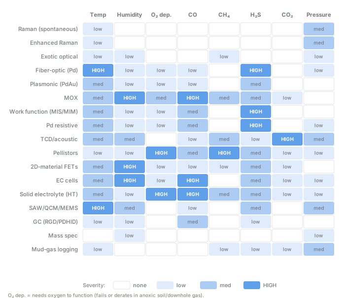
The technology × confounder matrix at a glance; severity blends response bias and poisoning. Quantitative coefficients live in each modality page; larger version on the charts page.

Cross-sensitivity & environment

Layer 1 by family. For electrochemical cells the dominant covariate is not steady-state temperature (compensated to ≤18–20 ppm zero drift [16][17]) but transients: rapid RH or T changes produce spurious spikes as the electrolyte’s outer diffusion layer re-equilibrates out of step with the bulk [19]. Pressure acts through the diffusion-limited current directly, so the GA5000 chamber test’s depressurization overestimation applies to any pumped method, where the pump itself creates a pressure transient at read time [20] (Electrochemical cells).

For MOX the structure is worse: RH dominates because water dissociatively chemisorbs, forming hydroxyls that both lower baseline resistance (mimicking a reducing gas) and occupy receptor-oxygen sites [22], compounding into the 25–40% long-term drift of a year-long dataset [26]. A MOX reading without an RH channel records H2 convolved with an unknown humidity state. O2 dependence adds a hypoxic-soil failure mode near active seeps: Nissha datasheets require >18% O2 [23][24] (MOX sensors).

For thermal conductivity the problem is inability to distinguish the analyte from interferents, because it measures one scalar and inverts assuming a known binary mixture, while soil gas is never binary. Via a linear Wassiljewa approximation [29][30], 1% CO2 gives ~−650 ppm H2-equivalent (masking), 1% CH4 ~+350 ppm (false-high), and 1% He ~+7,700 ppm, making He the largest interferent because it is co-generated with geologic H2. Humidity compounds non-monotonically, peaking near 40–60% RH (up to 2 vol.% error) and flipping sign within a single field day [28] (Thermal conductivity).

For Pd resistive the covariance is double: temperature affects kinetics (60–80 kJ/mol barrier, 10 K ≈ doubles speed [31]) and the α↔β thermodynamic equilibrium itself (van’t Hoff, $\Delta H\approx-36\pm1$ kJ/mol, $\Delta S\approx88\pm3$ J/mol·K [32]), so the calibration curve shifts, with one hybrid inverting outright (11.3%→8.3% from 25 to 100 °C) [33]. Humidity mostly slows kinetics reversibly [34], and pressure enters multiplicatively via Sieverts’ law, needing a total-P correction most 1-ATM vendor calibrations omit [35] (Palladium-resistive, Work-function devices).

Layer 2 by covariate. Soil moisture is the strongest single covariate, acting three ways at once: it sets gas-phase diffusivity and air-filled porosity, modulates the microbial sink, and at high saturation caps the flux via a high-interfacial-tension seal [6]. The same WA site swung 493 → 330 → 52 ppm across dry, intermediate, and post-rain periods [6], an order of magnitude from moisture alone. Barometric pressure is the hardest to disentangle because it acts on both layers: falling pressure drives genuine advective outgassing and independently biases the GA5000 high [20], and a single spot reading during a drop cannot separate the two. Temperature correlates diurnally but explains little variance ($r^2=0.13$) [7]; soil temperature at 1 m stays stable while air temperature swings, so the diurnal correlation likely proxies a barometric or biological cycle rather than being causal [6][7]. The microbial sink (~71% of the global atmospheric H2 sink, ~60 Tg/yr [38], active to −70 to −100 MPa [4]) essentially never switches off, while local nitrogen fixation adds a non-geologic positive near legumes and diazotroph-rich soils [4][39].

The joint problem. The hardest cases are collinear: one driver moves both layers the same direction. Falling pressure drives real advective release (Layer 2) while biasing an electrochemical cell high (Layer 1) [6][7][20]. Rising humidity after rain suppresses true flux by capping the soil (Layer 2) while producing a humidity-shock transient (Layer 1), possibly in the opposite direction. The only established ways to break the collinearity are multivariate/harmonic regression against independently logged covariates, and corroboration with an orthogonal proxy.

The 2023–2025 measurement-artifact controversy

Read through the covariance lens, this debate is a live Layer-1/Layer-2 confound. For artifacts: a 2025 study across 24 sub-circular depressions (83 holes, non-redrilled repeats) found drilling-induced artifacts up to 464 ppm at 85% of locations, only ~15% attributable to natural H2 [11], via “drill-bit metamorphism,” a mechanochemical process stronger in ultramafic than carbonate rock [12]. For genuine signal: MONHyTOR found post-installation peaks decaying exponentially with soil-type-dependent parameters (clay: high initial, slow decay; sand: low initial, fast decay), consistent with diffusion rather than a pure artifact [10], and telemetered PARHyS/WHALI/EVA recorded diurnal and multi-day pulses recurring over months, beyond any single drilling event [8][9][13].

What both sides now largely agree on

1. Single spot measurements immediately after drilling, without a settling period, are unreliable, especially in ultramafic/high-strength/low-moisture soils [11][12].
2. Pressure and humidity transients meaningfully bias at least one widely used field instrument at exactly the ppm-to-tens-of-ppm scale relevant to exploration [20].
3. Genuine natural seepage is corroborated by lithology-consistent decay kinetics, multi-month recurring cycles, and downhole neutron-log anomalies no soil-probe artifact can explain [10][8][9][13].
4. Best practice converges on percussion (not rotary) drilling, repeat measurement without redrilling, multi-week continuous monitoring, and mandatory co-logging of soil moisture, strength, and lithology alongside every H2 reading [7][11][12].

Summary matrix

Technology	Temperature	Humidity	Pressure	CO2/matrix	Poisoning (H2S/siloxane)	Primary mitigation
Electrochemical	Low–moderate (compensable, ≤20 ppm drift)	Moderate, transient-dominated	Moderate (depressurization → high bias)	Low (CO is the main gas interferent, not CO2)	H2S degrades working electrode over time	Co-log T/RH/P; avoid pumping transients at read time; periodic recalibration
MOX	High (~2× baseline swing)	Dominant covariate	Unquantified/unknown, flagged open question	Indirect (O2-dilution pathway)	Siloxane: 40–70% sensitivity loss within ~1 yr equivalent exposure; H2S: permanent baseline shift	Mandatory T/RH co-logging; periodic re-zeroing; screening role only
Thermal conductivity/TCD	High (~100× signal at 60 °C swing, uncompensated)	High, non-monotonic, sign-flipping	Pirani-regime devices only	He: severe false-high; CO2: false-low; CH4: false-high	None (no catalyst, no chemisorption)	Onboard T/RH/P compensation (MEMS parts); pair with independent He/CO2 channel
Pd resistive	High (kinetics + thermodynamic calibration shift)	Moderate, mostly reversible	High (Sieverts sqrt-law, needs total-P correction)	Low (CO2/CH4 held to ±4% in best devices)	H2S is the main poisoning risk; CO manageable via alloying	Thermal control/compensation; H2S scrubber pre-filter; alloy for CO tolerance
Catalytic pellistor (context)	Moderate	Low–moderate	Requires ≥~10–14% O2, fails in inert atmosphere	N/A (combustion-based)	Silicone/lead: permanent; H2S/halogens: reversible inhibition	Not usable in anoxic settings at all

See Catalytic pellistors for the fifth row’s derivation.

Use for geologic H₂

Field verdict

No raw reading from any family is interpretable on its own. The covariance structure is the quantitative justification for why the field community standardized on electrochemical cells as the primary quantitative channel (GA5000, MONHyTOR, PARHyS, WHALI/EVA all use amperometric cells) [7][10][20][8][9][13], not because they are covariate-free but because their covariate magnitudes at ppm-to-low-percent concentrations are smaller and better characterized than MOX’s ~2× T-driven swing or TCD’s up-to-+7,700-ppm He interference. Every soil-gas reading needs simultaneous logging of soil temperature at probe depth, volumetric soil moisture, barometric pressure and its rate of change, and gas-line RH, plus where affordable a co-measured proxy gas (He, CO2, CH4) to catch the interferents that most threaten the chosen sensor.

Soil-gas surveys. Covariate logging matters most here: without it, a spot reading cannot distinguish a real seep suppressed by rain from a dry-season non-event inflated by depressurization. Minimum protocol: percussion drilling, a settling period, a repeat reading to test exponential decay versus a stable/rising signal, and moisture/temperature/pressure logging at the same depth and time [7][11][12].

Downhole/borehole logging. Layer 1 covariance gets worse: deep formation T/P (100–230+ °C, tens of MPa) sits far outside every family’s published covariate envelope, all characterized near 1 ATM and room temperature; extrapolating Pd’s Sieverts correction, MOX’s O2 dependence, or TCD’s Pirani sensitivity to those conditions is unsupported. Layer 2 is comparatively less of a problem at depth, since the signal is well above ppm background and the barometric/moisture/microbial mechanisms are near-surface. So downhole measurement today avoids the sensor-covariance problem entirely, using indirect wireline neutron-porosity logs [15] or bringing a physical sample to surface for gas chromatography or mass spectrometry under controlled T/P (Downhole deployment).

Continuous monitoring stations. The interpretive framework is most actionable here: a station logging H2 with the four covariates for several weeks (ideally a full season) is the only configuration in which the harmonic/multivariate regression can separate a genuine multi-day pulse from drilling artifacts, pumping artifacts, humidity shock, and the diurnal cycle. Every rigorous “real signal” claim reviewed (MONHyTOR’s lithology-consistent decay [10], PARHyS/WHALI/EVA’s multi-month structure [8][9][13]) rests on a continuous record long enough for exactly this decomposition, never a single spot reading (Soil-gas surveys, Calibration & QA/QC).

Vendors & products

Instruments and reference parts behind the quantitative artifacts cited above:

Vendor/product	Role in this dossier	Key quantitative artifact	Ref
Geotech/QED GA5000	Field-standard electrochemical multi-gas analyzer; subject of the only controlled T/P/RH/CO chamber characterization found in this session	Depressurization (500–1400 mbar sweep) → overestimation bias at fixed 50 ppmv H2	[20][40]
ISTerre/Grenoble MONHyTOR probe	Buried non-pumping continuous H2/T probe, 1 m depth	Exponential post-installation decay, soil-type-dependent $\alpha$	[10]
ENGIE PARHyS	Telemetered continuous soil-gas station, ~100 units deployed, Brazil	6–8 months of diurnal-cycle-resolved monitoring	[8][9]
Axiom Sensing WHALI (pumped) / EVA (passive)	Autonomous continuous loggers, Western Australia	Diurnal H2 flux correlated with barometric pressure	[13]
Figaro TGS821	MOX reference part for T/RH baseline-swing coefficients	~2× $R_s/R_0$ swing, −20…+50 °C	[21]
Nissha FIS SB-19-00 / SP-19-01	MOX reference parts for O2-dependency documentation	>18% O2 minimum stated on datasheet	[23][24]
Winsen ME3-H2 / Membrapor H2/M-1000	Electrochemical reference parts for T-drift specs	≤20 ppm / ≤18 ppm zero drift over stated T ranges	[16][17]
Sensirion STC31 / STC31-C	MEMS thermal-conductivity parts; subject of a controlled humidity-error study	Up to 2 vol.% H2-equivalent RH-driven error	[28][41]
H2scan HY-OPTIMA series	Pd-based process analyzer; source of Sieverts-law pressure-correction guidance	Calibrated at 1 ATM; pressure compensation recommended off-ATM	[35]
Alphasense H2-AF / H2-BF	Electrochemical sensor elements cited for T/RH-limit specifications	≤0.7 ppm RMS noise, −30…+50 °C, 15–90% RH rated	[42]
WatchGas / Industrial Scientific / Crowcon	Source of published cross-interference and T-dependent cross-sensitivity tables	H2-driven CO false reading 18/36/54 ppm at 10/20/30 °C	[18][43]

Open questions

1. No published downhole-relevant covariate data exists for any family here; every coefficient was measured near 1 ATM and room-to-moderate temperature. Extrapolating Sieverts pressure correction, MOX O2 dependence, or TCD Pirani behavior to 100–230 °C and tens of MPa is unsupported, a research gap, not benign.
2. No quantitative literature was found on TCD sensitivity to H2S (a sibling dossier flags “small, uncertain-sign bias, unverified magnitude”). If a TCD channel is considered for an H2S-co-evolving site, close this gap experimentally.
3. The barometric-pumping equations are at the level of general vadose-zone theory, not a fully verified H2-specific source; a follow-up with the barometric-pumping/radon literature would give hard numbers (advective velocity per mbar/hr) rather than direction-of-effect.
4. The regression toolkit in the primary geo-H2 literature is unsophisticated relative to adjacent fields (radon ML anomaly detectors [44], low-cost methane-network calibration [45]); an opportunity for Hestia to differentiate on interpretation methodology (Kalman-filter or harmonic-regression pipeline against co-logged covariates).
5. No commercial off-the-shelf continuous H2 station with integrated multi-covariate logging exists; PARHyS, MONHyTOR, and WHALI/EVA are bespoke builds, so treat buy-vs-build as an open decision.
6. The author list for the drilling-induced hydrogen paper [12] (Pengg, Misch, Tari, Sachsenhofer, Zach, Stranzl) was confirmed by cross-referencing during the 2026-07 verification pass; resolved.
7. Alphasense’s full-PDF datasheet resisted automated extraction; the T/RH numbers for [42] came through as search snippets, worth re-verifying against the primary PDF before treating as load-bearing. (Membrapor’s zero-drift figure for [16] has since been confirmed by direct PDF extraction.)

Related pages

• Geologic context: the transport-physics and drilling-artifact companion this page’s covariate math builds on
• Soil-gas surveys: the field protocol that most needs the covariate-logging discipline here
• Downhole deployment: why Layer 1 covariance gets worse, not better, at depth
• Calibration & QA/QC: the operational procedures that implement covariate correction
• Electrochemical cells: the default soil-gas workhorse, with the best-characterized (not smallest) covariate structure
• MOX sensors: the largest, least-correctable humidity covariate
• Thermal conductivity & acoustic sensors: the mixing-rule physics behind the He/CO2/CH4 interference table
• Palladium-resistive sensors and Work-function devices: H2-specific solid-state alternatives with their own T/P calibration-shift problems
• Catalytic pellistors: the O2-dependence and poisoning mechanisms in the summary matrix
• FET / 2D-material sensors: an emerging route whose covariance is not yet field-characterized
• Solid-electrolyte high-temperature sensors: a covariate regime opposite to near-surface soil gas
• SAW / QCM / MEMS resonant sensors: mechanical transduction with its own T/P resonance drift
• Plasmonic metamaterials: an emerging optical route for interferent-resistant transduction
• Gas chromatography, Mass spectrometry, and Mud-gas logging: the corroboration and physical-sampling methods that break Layer-1/Layer-2 collinearity
• Why H2 is hard: the selection-rule framing behind why no transduction physics escapes this covariance

References

Full reference list (45 entries)

[1] Massman, W.J. (1998). “A review of the molecular diffusivities of H2O, CO2, CH4, CO, O3, SO2, NH3, N2O, NO, and NO2 in air, O2 and N2 near STP.” Atmospheric Environment. https://www.sciencedirect.com/science/article/abs/pii/S1352231097003919

[2] Ehhalt, D.H., Rohrer, F. (2013). “Deposition velocity of H2: a new algorithm for its dependence on soil moisture and temperature.” Tellus B: Chemical and Physical Meteorology 65(1), 19904. DOI: 10.3402/tellusb.v65i0.19904. https://b.tellusjournals.se/articles/10.3402/tellusb.v65i0.19904

[3] Yver, C., Schmidt, M., Bousquet, P., Ramonet, M. (2011). “Measurements of molecular hydrogen and carbon monoxide on the Trainou tall tower.” Tellus B: Chemical and Physical Meteorology 63(2) (seasonal amplitude ~45 ppb, nighttime depletion, radon-tracer-method deposition velocity ~2.6×10⁻² cm/s). DOI: 10.1111/j.1600-0889.2010.00520.x. https://b.tellusjournals.se/articles/10.1111/j.1600-0889.2010.00520.x

[4] Reji, L., Bertagni, M.B., Paulot, F., Qin, Q., Zhang, X. (2025). “Global implications of a low soil moisture threshold for microbial hydrogen uptake.” Nature Communications. DOI: 10.1038/s41467-025-67208-3. https://pmc.ncbi.nlm.nih.gov/articles/PMC12804893/

[5] “Barometric-pumping controls fugitive gas emissions from a vadose zone natural gas release.” PMC6773692. https://www.ncbi.nlm.nih.gov/pmc/articles/PMC6773692/

[6] Davies, K. et al. (2024). “A natural hydrogen seep in Western Australia: Observed characteristics and controls.” Science and Technology for Energy Transition. DOI: 10.2516/stet/2024043. https://www.stet-review.org/articles/stet/full_html/2024/01/stet20240139/stet20240139.html

[7] Davies, K., Haines, P.W., Thomas, C., Normore, L. (2025). “Natural hydrogen soil gas emissions near Harvey, Perth Basin: a comparative study of survey methods.” Science and Technology for Energy Transition 80, 46. DOI: 10.2516/stet/2025026. https://www.stet-review.org/articles/stet/full_html/2025/01/stet20250031/stet20250031.html

[8] Moretti, I. et al. (2021). “Long-term monitoring of natural hydrogen superficial emissions in a Brazilian cratonic environment. Sporadic large pulses versus daily periodic emissions.” International Journal of Hydrogen Energy. https://www.sciencedirect.com/science/article/abs/pii/S0360319920341987; https://www.researchgate.net/publication/347274944

[9] ENGIE Research & Innovation. “Is natural hydrogen of the ‘fairy circles’ the new eldorado?” (PARHyS deployment description, ~100 units, São Francisco basin, Brazil). https://innovation.engie.com/en/articles/detail/is-natural-hydrogen-the-new-eldorado/26061/1/3

[10] Adjie, N., Bordes, C., Brito, D., Nasri, D., Normandin, É. (2025). “In-soil hydrogen concentration monitoring using MONHyTOR: application for natural hydrogen exploration.” Advances in Geosciences 67, 57–64. DOI: 10.5194/adgeo-67-57-2025. https://adgeo.copernicus.org/articles/67/57/2025/

[11] Davies, K., Josse, R., Frery, E., Esteban, L., Keshavarz, A., Iglauer, S. (2025). “Distinguishing drilling-induced artifacts from naturally occurring hydrogen in soil gas surveys: Insights from sub-circular depressions.” International Journal of Hydrogen Energy 109, 1230–1240. https://www.sciencedirect.com/science/article/pii/S0360319925006597

[12] Pengg, A., Misch, D., Tari, G., Sachsenhofer, R.F., Zach, C., Stranzl, C. (2025). “Drilling-induced hydrogen: A challenge for natural hydrogen exploration.” International Journal of Hydrogen Energy, vol. 149, art. 150091. Author list confirmed via independent cross-referencing (ResearchGate listing and Montanuniversität Leoben author-affiliation records) during 2026-07 citation verification; not directly visible on the paywalled ScienceDirect abstract page. https://www.sciencedirect.com/science/article/pii/S0360319925030885

[13] Axiom Sensing. WHALI/EVA autonomous logger system description and field-deployment figures. https://www.axiomsensing.com/ ; https://www.researchgate.net/figure/cH2-for-the-WHALI-and-EVA-autonomous-logging-units-for-the-February-2023-monitoring_fig7_381304297

[14] Gelman, S.E., Hearon, J.S., Ellis, G.S. (2025). “Prospectivity mapping for geologic hydrogen.” USGS Professional Paper 1900. DOI: 10.3133/pp1900. https://pubs.usgs.gov/publication/pp1900

[15] Maiga, O., Deville, E., Laval, J., Prinzhofer, A., Diallo, A.B. (2023). “Characterization of the spontaneously recharging natural hydrogen reservoirs of Bourakebougou in Mali.” Scientific Reports. DOI: 10.1038/s41598-023-38977-y. https://pmc.ncbi.nlm.nih.gov/articles/PMC10363119/

[16] Membrapor AG. “Hydrogen Gas Sensor H2/M-1000” datasheet (zero shift specification, 18 ppm over +20…+40 °C, per search-indexed content). https://www.membrapor.ch/sheet/Hydrogen-Gas-Sensor-H2-M-1000.pdf

[17] Winsen Electronics. “ME3-H2 Electrochemical Hydrogen Gas Sensor.” Product page. https://www.winsen-sensor.com/sensors/h2-sensor/me3-h2.html

[18] WatchGas. “Application Note 4 — Sensor Technical Data Summaries,” Carbon Monoxide (CO) – Low Hydrogen Interference table (T-dependent false readings, 18/36/54 ppm at 10/20/30 °C for 900 ppm H2). Corrected during 2026-07 citation verification — the MSA Safety bulletin previously cited here does not contain this data. https://watchgas.com/app/uploads/2023/09/Technical-Note-4-v1.9.pdf

[19] “Considerations of Thermodynamics and Kinetics for the Effects of Relative Humidity on the Electrolyte in Electrochemical Toxic Gas Sensors.” ACS Sensors (2021). DOI: 10.1021/acssensors.1c01339.

[20] Auclair, S., Lefeuvre, N., Dutoit, H., Donzé, F-V., Truche, L. (2024). “Assessing the Portable Gas Analyzer GA5000 for Accurate H2 Monitoring in Geological Exploration.” Geonum Ed. https://hal.science/hal-04861335; https://www.researchgate.net/publication/385938959

[21] Figaro Engineering Inc. “TGS 821 – Special Sensor for Hydrogen Gas,” product datasheet. https://www.figarosensor.com/product/docs/TGS821.pdf

[22] “Reducing Humidity Response of Gas Sensors for Medical Applications: Use of Spark Discharge Synthesis of Metal Oxide Nanoparticles.” PMC6111941. https://pmc.ncbi.nlm.nih.gov/articles/PMC6111941/

[23] Nissha FIS, Inc. “FIS Gas Sensor SB-19-00 for Hydrogen Detection,” specifications. https://www.fisinc.co.jp/en/common/pdf/SB1900E.pdf

[24] Nissha FIS, Inc. “FIS Gas Sensor SP-19-01 for Hydrogen Detection,” specifications. https://www.fisinc.co.jp/en/common/pdf/SP1901E_P.pdf

[25] “Correction Model for Metal Oxide Sensor Drift Caused by Ambient Temperature and Humidity.” PMC9101743. https://pmc.ncbi.nlm.nih.gov/articles/PMC9101743/

[26] “Long-term drift behavior in metal oxide gas sensor arrays: a one-year dataset from an electronic nose.” Scientific Data (2025). https://www.nature.com/articles/s41597-025-05993-8

[27] “A Robust Miniaturized Gas Sensor for H2 and CO2 Detection Based on the 3ω Method,” PMC8780541. https://pmc.ncbi.nlm.nih.gov/articles/PMC8780541/ ; also MDPI Sensors 22(2):485. https://www.mdpi.com/1424-8220/22/2/485 (does not support the claim)

[28] Emperhoff, S., Eberl, M., Dwertmann, T., Wöllenstein, J. (2024). “On the Influence of Humidity on a Thermal Conductivity Sensor for the Detection of Hydrogen.” Sensors 24(9), 2697. DOI: 10.3390/s24092697. https://pmc.ncbi.nlm.nih.gov/articles/PMC11086256/

[29] Brokaw, R.S. (1965). “Viscosity and Thermal Conductivity of Gas Mixtures. Accuracy of Some Empirical Formulas.” Journal of Chemical Physics 42(7), 2533 (Wassiljewa equation performance for binary vs. multicomponent gas mixtures). https://ui.adsabs.harvard.edu/abs/1965JChPh..42.2533B/abstract

[30] IDAES documentation. “Wassiljewa-Mason-Saxena Method for Low-pressure Gas Mixture Thermal Conductivity.” https://idaes-pse.readthedocs.io/en/2.5.0/explanations/components/property_package/general/transport_properties/thermal_conductivity_wms.html

[31] Darmadi, I., Nugroho, F.A.A., Langhammer, C. (2020). “High-Performance Nanostructured Palladium-Based Hydrogen Sensors—Current Limitations and Strategies for Their Mitigation.” ACS Sensors 5(11), 3306–3327. DOI: 10.1021/acssensors.0c02019. https://pmc.ncbi.nlm.nih.gov/articles/PMC7735785/

[32] “Measurement of Palladium Hydride and Palladium Deuteride Isotherms Between 130 K and 393 K.” https://www.researchgate.net/publication/342758683_Measurement_of_Palladium_Hydride_and_Palladium_Deuteride_Isotherms_Between_130_K_and_393_K

[33] Yan, S., Cao, Y., Su, Y., Huang, B., Chen, C., Yu, X., Xu, A., Wu, T. (2025). “Hydrogen Sensors Based on Pd-Based Materials: A Review.” Sensors 25(11), 3402. DOI: 10.3390/s25113402. https://pmc.ncbi.nlm.nih.gov/articles/PMC12157283/

[34] Ngo, T.A., Magar, A.T., Pham, M.T., et al. (2025). “Fullerene-decorated PdCo nano-resistor network hydrogen sensors with sub-second response and parts-per-billion detection at room temperature.” Nature Communications 17. DOI: 10.1038/s41467-025-67708-2. https://pmc.ncbi.nlm.nih.gov/articles/PMC12847907/

[35] H2scan Corporation. “HY-OPTIMA Series In-Line Hydrogen Process Monitor” product/FAQ pages (Sieverts partial-pressure device, 1 ATM calibration, pressure-compensation guidance, per-model CO/H2S tolerance). https://h2scan.com/product/hy-optima-5000/ ; https://h2scan.com/resource-gallery/faqs/

[36] Novelli, P.C., Lang, P.M., Masarie, K.A., Hurst, D.F., Myers, R., Elkins, J.W. (1999). “Molecular hydrogen in the troposphere: Global distribution and budget.” Journal of Geophysical Research 104(D23), 30427–30444. DOI: 10.1029/1999JD900788.

[37] “First detection of industrial hydrogen emissions using high precision mobile measurements in ambient air.” Scientific Reports, PMC11480439. https://pmc.ncbi.nlm.nih.gov/articles/PMC11480439/

[38] Paulot, F., Pétron, G., Crotwell, A.M., Bertagni, M.B. (2024). “Reanalysis of NOAA H2 observations: implications for the H2 budget.” Atmospheric Chemistry and Physics 24, 4217–4229. DOI: 10.5194/acp-24-4217-2024. https://acp.copernicus.org/articles/24/4217/2024/

[39] Bertagni, M.B. et al. (2021). “Moisture Fluctuations Modulate Abiotic and Biotic Limitations of H2 Soil Uptake.” Global Biogeochemical Cycles. https://agupubs.onlinelibrary.wiley.com/doi/full/10.1029/2021GB006987

[40] Geotech/QED Environmental Systems. “GA5000 Portable Gas Analyzer” specification pages. https://www.qedenv.com/products/portable-gas-analyzer-ga5000/

[41] Sensirion AG. “Datasheet STC31 - CO2 Sensor Based on Thermal Conductivity Measurement Principle” and STC31-C design guide (RH/O2 low-cross-sensitivity mode). https://sensirion.com/media/documents/7B1D0EA7/61652CD0/Sensirion_Thermal_Conductivity_Datasheet_STC31_D1_1.pdf; https://sensirion.com/products/catalog/STC31-C

[42] Alphasense (AMETEK). “Hydrogen Sensors (H2)” product line, H2-AF specification page. https://www.alphasense.com/products/view-by-target-gas/hydrogen-h2; https://store.alphasense.com/h2-af/

[43] Industrial Scientific. “Electrochemical Gas Sensor Cross Interference Table.” https://www.indsci.com/en/blog/electrochemical-sensor-cross-interference-table

[44] “Delegated Regressor, A Robust Approach for Automated Anomaly Detection in the Soil Radon Time Series Data.” PMC7033208. https://www.ncbi.nlm.nih.gov/pmc/articles/PMC7033208/

[45] “Laboratory and field evaluation of a low-cost methane sensor and key environmental factors for sensor calibration.” PMC10100561. https://www.ncbi.nlm.nih.gov/pmc/articles/PMC10100561/