Figures of merit: how to compare any two H2 sensors honestly

Summary

“Which H₂ sensor is better?” has no answer until you fix the axis of comparison. A Raman analyzer resolves 190 ppm with near-certain gas identification; a $2 metal-oxide bead claims sub-ppm detection and loses the claim when humidity swings 20 points. Neither number is a lie; both are incomplete without knowing what was held fixed while measuring.

A figure of merit (FoM) is a named, standardized comparison axis (how sensitive, how selective, how fast, how stable) that puts sensors built on different physics (How sensors differ) on the same footing. This page defines the fourteen FoMs used throughout this wiki: meaning, formula, worked arithmetic, and the conditions each number silently assumes. The one idea to carry through: every figure of merit is a claim measured under conditions, and the conditions are what the spec sheet leaves out.

Context numbers used throughout

Atmospheric H₂ background ≈ 0.53 ppm (recent network means fall in the 531–553 ppb range) [1]; geologic H₂ soil-gas anomalies span roughly 1 ppm to percent level; H₂’s lower explosive limit (LEL) = 4 vol% (40,000 ppm). This page is the compute-it-yourself companion to Reading the specs, which walks the same material through real vendor datasheets line by line.

The model behind every spec line

A sensor reports a noisy, drifting, environmentally nudged stand-in for the true concentration:

$$R(t) \approx R_0(t) + S(t)\,C_{H_2}(t) + \sum_i \kappa_i(t)\,C_i(t) + n(t)$$

The reading $R$ is a baseline $R_0$ (the zero-gas output), plus true concentration $C_{H_2}$ times sensitivity $S$, plus every interferent gas $i$ weighted by its cross-sensitivity coefficient $\kappa_i$, plus random noise $n$. Every FoM below names one term or one behavior of this equation: sensitivity is $S$, limit of detection compares $n$ to $S$, selectivity is the size of $\kappa_i$, drift is $R_0$ and $S$ changing with time. Read a spec line as “one term, measured one particular way” and a datasheet becomes a short list of checkable claims.

Sensitivity (S)

The calibration slope: how much the signal moves per unit of H₂.

$$S \equiv \frac{\partial(\text{signal})}{\partial(\text{concentration})}$$

Units are family-specific (nA/ppm for an electrochemical cell, a resistance ratio for a chemiresistor, pm/% for a fiber’s wavelength shift, Hz/ppm for a quartz crystal) because “signal” is physically different in each family (Gas vs. aqueous sensing). Raw slopes across unlike units cannot be compared until each is divided by its own noise floor, which is what LOD does.

Worked example. The Alphasense H2-AF cell reports 10–40 nA/ppm at 400 ppm, 23°C [2]. At −20°C it delivers 10–25% of its 20°C output; at 50°C, 220–275% [2]. The extremes span $275\%/10\%=27.5$: the same hardware can swing 27.5× in raw sensitivity across a realistic field temperature range. “10–40 nA/ppm” without a temperature qualifier silently assumes 23°C.

Absolute vs. relative. Normalizing the slope by the baseline, $(\partial R/\partial C)/R_0$, removes unit-to-unit zero-point spread: Figaro’s TGS2600 shows a 9× baseline-resistance spread (10–90 kΩ) but only a 2× spread in the normalized ratio (0.3–0.6) [3]. Calibrate batches against the normalized number.

A vendor-quoted $S$ is one calibration point on a small sample; re-verify it on the unit in hand.

Limit of detection (LOD)

The smallest concentration reliably distinguished from zero. Three different procedures share the name:

(a) IUPAC 3σ, the metrological standard [4]:

$$\mathrm{LOD} = \frac{k\,\sigma_{blank}}{S}, \qquad k=3$$

At $k=3$ the false-positive rate is ≈0.135% under Gaussian noise, a real confidence statement. A 2024 methodology paper measured controlled-chamber zero-air noise of <500 pA (1.6 ppb-equivalent) and derived $\mathrm{LOD}=3\times1.6=4.8$ ppb [5]; the controlled chamber is doing most of the work in that number.

(b) SNR = 1. Sets $k=1$: an LOD exactly 3× smaller (more optimistic) on identical noise, with no confidence statement.

(c) Allan-deviation floor, the averaging-aware convention. White noise shrinks with averaging time as $\sigma(\tau)\propto\sigma(\tau_0)\sqrt{\tau_0/\tau}$, but at long $\tau$ drift dominates and precision worsens. The Allan variance [6],

$$\sigma_A^2(\tau) = \frac{1}{2(M-1)}\sum_{i=1}^{M-1}\left(\bar y_{i+1}(\tau)-\bar y_i(\tau)\right)^2$$

locates the true floor and best integration time $\tau^*$ at the minimum of $\sigma_A(\tau)$. It is the only convention that answers “if I dwell 30 s vs. 5 min per station, what is my real noise floor?”

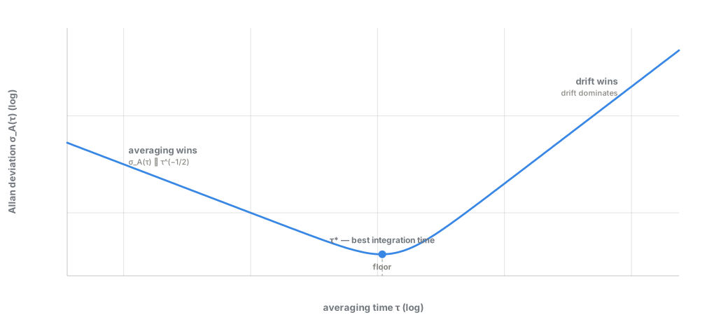
Schematic, not measured data: averaging helps until drift takes over, and τ marks the crossover.*

Worked example: one dataset, two answers. Using Alphasense’s <0.7 ppm RMS noise [2] as $\sigma_{blank}$: IUPAC 3σ gives $3\times0.7 =$ 2.1 ppm; SNR = 1 gives 0.7 ppm. Exactly 3× apart by construction, which is why this wiki lists electrochemical-cell LOD as a range (0.5–2 ppm) rather than one number.

LOD is a different quantity from resolution (below); the two are often conflated.

Limit of quantification (LOQ)

LOD answers “is gas present?”; LOQ answers “can I trust a number for how much?”, conventionally where relative uncertainty drops to ≤10%:

$$\mathrm{LOQ} \approx \frac{10\,\sigma_{blank}}{S}$$

Both the IUPAC and the pharmaceutical (ICH Q2) conventions use this 10× multiplier, making LOQ $10/3\approx3.3\times$ the matching IUPAC LOD [7].

Worked example. Same dataset: $\mathrm{LOQ}=10\times0.7=7$ ppm. A 3 ppm reading is detectable but not quantifiable to ±10%: the defensible statement at 3–7 ppm is “gas is present,” not “3.0 ± 0.3 ppm.” Treating any above-LOD reading as quantitative is the standard mistake.

Selectivity and cross-sensitivity (K_ij)

How much the sensor mistakes interferent $j$ (CO, CH₄, H₂S, humidity) for target $i$:

$$K_{ij} = \frac{S_j}{S_i}$$

traced to the IUPAC ion-selective-electrode framework [8]. Overall selectivity is $1/\max_j(K_{ij})$: as good as the worst interferent, not the average.

Worked example. Two electrochemical H₂ cells under the same category label: Alphasense H2-AF, CO cross-sensitivity <2% [2], so selectivity $=1/0.02=50$; Membrapor H2/M-1000, ~60–80% [9], so $1/0.70\approx1.4$. A ~35× difference ($50/1.4\approx36$) driven by an inlet filter and catalyst choice invisible from the product name.

Cross-sensitivity is a single-concentration snapshot: “CO <2% at 400 ppm CO” says nothing at 4,000 ppm or during simultaneous CO+H₂S exposure. Helium & co-tracers and Isotopes & fingerprinting cover independent confirmation paths.

Response and recovery time

Response time is how fast the output follows a concentration step; recovery, usually slower and less reported, is the return to baseline. For a single first-order process with time constant $\tau$ (fair for diffusion-limited electrochemical cells, poor for MOX/catalytic surface kinetics):

$$C(t)=C_{\text{final}}(1-e^{-t/\tau})\implies t_x=-\tau\ln\!\left(1-\frac{x}{100}\right)$$

so $t_{50}\approx0.693\tau$ and $t_{90}\approx2.303\tau$. IEC 60079-29-1 uses both as certification pass/fail criteria [10].

Worked example. Single-pole kinetics require $t_{50}/t_{90} = \ln2/\ln10\approx0.301$. A sheet quoting 10 s / 35 s gives 0.286, close enough to trust; 10 s / 200 s gives 0.05, signaling a long non-exponential tail (adsorption saturation, thick-coating diffusion) that a single-$\tau$ extrapolation would mis-model.

Recovery is desorption-governed; MOX chemiresistors document recovery constants measurably larger than response constants [3]. A sheet reporting only $t_{90}$ tells the easier half.

Dynamic range and linear range

Dynamic range is the span with usable output; linear range is the narrower span where one slope $S$ applies.

$$N_{\text{decades}}=\log_{10}\!\left(\frac{C_{\max}}{C_{\min}}\right)$$

Worked example. Alphasense H2-AF: warranted 2,000 ppm range and IUPAC LOD ≈2.1 ppm give $\approx3.0$ decades. The linearity comes from the diffusion-limited current $i_L=nFAD\,C_\infty/l$ [11] (Electrochemical cells), where every term but concentration is a geometric constant.

MOX, work-function, and FET sensors (MOX sensors, Work-function devices, FET & 2D materials) are intrinsically log-linear; plotting them on linear axes makes the low end look artificially flat.

Resolution vs. LOD

Resolution is the smallest increment the readout electronics can register, a property of the ADC/display/firmware chain, not the noise-limited floor.

Worked example. Membrapor states its <2.0 ppm resolution is “electronics dependent” [9]: the same cell with a different amplifier/ADC reports a different resolution while the chemistry’s LOD is unchanged. Comparing “0.7 ppm” vs. “2.0 ppm” across vendors may compare readout boards, not chemistries. The dangerous direction is a display finer than the true noise floor (“0.1 ppm” beside a real 2 ppm floor), which invites over-reading.

Accuracy, precision, repeatability, reproducibility

Four names for terms of one bias–variance decomposition:

$$\hat x = x_{\text{true}} + \underbrace{b(T,RH,P,t)}_{\text{bias}\Rightarrow\text{accuracy}} + \underbrace{\varepsilon,\ \varepsilon\sim\mathcal N(0,\sigma_{\text{rep}}^2)}_{\text{random error}\Rightarrow\text{precision}}$$

Accuracy is bias $b$ against a certified reference. Precision is the spread of repeats, regardless of centering: a sensor can be precise and badly biased. Repeatability is precision under fixed conditions; reproducibility is the spread across units and conditions, rarely reported because it needs a population of units.

Worked example: a full uncertainty budget per the GUM [12]. A field cell with calibration-reference uncertainty $u_1=3\%$ of reading, 8-month post-fill drift $u_2=0.7\%$, noise floor $u_3=0.3$ ppm, and a 3-day-old span check under a documented 1 ppm/day drift bound (rectangular distribution: $u_4=3/\sqrt3\approx1.7$ ppm). At a 5.0 ppm reading:

$$u_c=\sqrt{0.15^2+0.035^2+0.3^2+1.7^2}\approx1.73\text{ ppm},\quad U=2u_c\approx3.5\text{ ppm}\ (k{=}2,\ {\sim}95\%\text{ coverage})$$

The dominant term by nearly an order of magnitude is time-since-last-calibration drift, not reference-gas quality: money goes further on frequent field re-zero/span checks than on a better cylinder. See Calibration, drift & QA/QC. And “<2% repeatability” [9] says nothing about bias without an independent calibration statement.

Drift

Baseline (zero) drift and span (sensitivity) drift are independent processes:

$$R_0(t)=R_0(0)+d_Z t+w_Z(t),\qquad S(t)=S(0)(1+d_S t)+w_S(t)$$

Worked example. Alphasense reports zero drift <20 ppm/yr and marks sensitivity drift “nd” [2]; Membrapor reports span drift <15%/yr with zero drift folded into an overall figure [9]. Uncorrected for 2 years, 15%/yr leaves sensitivity at $(0.85)^2\approx0.72$ of original, requiring a $1/0.72\approx1.39$ (39%) correction no factory curve knows to apply.

“nd” is unmeasured, not zero. Both rates run per unit time, not per unit use; the clock ticks in the warehouse.

Hysteresis

Path dependence: does 5 ppm read the same rising toward it as falling back to it? Distinct from drift; hysteresis can appear with zero drift.

Worked example. Bulk palladium below the α↔β critical temperature (≈292–295°C) has a first-order transition whose absorption branch sits above the desorption branch, a two-branch equilibrium rather than a kinetic artifact: $R/R_0\approx1.52$ on absorption vs. ≈1.57 on desorption [13][14], a width of ~0.05 in $R/R_0$. Gold alloying (~25 at%) or particle sizes below ~10 nm mitigate it; see Palladium resistive.

Hysteresis is invisible unless both ramp directions are measured; a rising-only test cannot see it.

Power, warm-up, and operating envelope

Power and warm-up. For MOX, catalytic, and thermal-conductivity families, power is heater-dominated (a surface held at 200–550°C), and a freshly powered element does not match its calibration curve until warm. Figaro’s continuous TGS2600 draws ~210 mW; the pulsed TGS8100, same chemistry, ~15 mW, a ~14× reduction [3] and roughly 14× the battery life at a station. Pellistors are comparable: SGX’s MP-7217 draws 135–230 mW [15], Honeywell’s CAT25 similar [16]. See Thermal conductivity & acoustic sensors and Catalytic pellistors.

Operating envelope. Three nested domains: storage (survives unpowered) ⊃ operating (produces output) ⊃ compensated (stated accuracy holds):

$$C_{\text{reported}}=C_{\text{raw}}\cdot f_T(T)\cdot f_{RH}(RH)\cdot f_P(P)$$

Outside the compensated domain the corrections are extrapolated or absent while the device keeps producing numbers. Alphasense’s operating range is −30 to 50°C, yet the 27.5× sensitivity swing computed earlier sits entirely inside it [2]: a deployment can stay inside “operating” while accuracy is void. Downhole deployment and solid-electrolyte sensors face the same trap from opposite temperature directions.

Lifetime, calibration interval, and poisoning

Lifetime is time to a defined signal loss; calibration interval is the re-check cadence; poisoning is permanent sensitivity loss from a named exposure, as opposed to reversible interference. Anchors: Alphasense warrants 24 months to 80% signal; Membrapor carries a 3-year warranty and 3–5 year expected life [2][9]; pellistors need daily bump tests and up to 4×/year recalibration in safety-critical service [15].

Poisoning

Poisoning is a common-substance risk, not an exotic one: Figaro’s caution list names hair-grooming products and silicone rubber/putty for MOX elements [17]; ISO 26142 defines a standardized poison-test protocol, and resistance to it is strongly model-dependent across catalytic, MOX, and electrochemical designs [18].

“Maintenance-free” marketing is not a warranted drift-rate number.

The trade-off triangles

Sensitivity, selectivity, and stability draw on the same finite resource: the surface or bulk chemistry available to interact with H₂. A catalyst engineered for maximum H₂ affinity has fewer, more reactive, more exposed sites, which are exactly the sites most vulnerable to poisoning and drift and least able to discriminate H₂ from CO. Porous, poison-resistant pellistor beads are documented as less sensitive than solid-surface beads for this reason (Catalytic pellistors). There is no fourth axis; every fix for one vertex taxes the others.

The second triangle is LOD–response time–power: lowering LOD by averaging longer costs response speed; lowering it with a hotter surface or brighter source costs power. Cavity-enhanced and multipass optics buy orders of magnitude of LOD over spontaneous Raman precisely by spending integration time or optical power (Enhanced Raman).

Selectivity-normalized LOD. The effective field LOD is the lab LOD degraded by the interferents actually present:

$$\mathrm{LOD}_{\text{eff}}\approx\mathrm{LOD}_{\text{lab}}+K_{ij}\,C_j$$

Worked example. Membrapor ($K_{CO}\approx0.70$) in air with a 5 ppm CO background (plausible near combustion sources or mud-gas logging equipment) carries a $0.70\times5=3.5$ ppm bias, comparable to a genuine 5 ppm anomaly. Alphasense ($K_{CO}<0.02$) carries $0.02\times5=0.1$ ppm. Re-derive every headline LOD against the interferent background expected on site.

From fourteen universal ideas to every modality

Every specialized FoM on the technology pages is one of the fourteen ideas above applied to that family’s signal; each dossier’s “Figures of merit” section points back here.

Family	Specific FoM	Formula	Universal idea it specializes
Electrochemical cells	Amperometric sensitivity	$S=i_L/C_\infty=nFAD/l$	Sensitivity, a genuine constant across 2–4 decades
MOX sensors	Power-law exponent	$S\propto P^\beta$ [19]	Dynamic/linear range; $S$ varies with concentration
Work-function devices	Work-function shift	$\Delta\Phi$	Sensitivity
Palladium resistive	Fractional resistance change	$\Delta R/R$ (up to ≈0.8–0.87)	Sensitivity, paired with hysteresis
Catalytic pellistors	Bridge sensitivity	mV per % LEL	Sensitivity, plus poison resistance
SAW/QCM/MEMS	Sauerbrey mass sensitivity	$\Delta f=-C_f\Delta m$, $C_f=2f_0^2/(A\sqrt{\rho_q\mu_q})$	Sensitivity, scaling as $f_0^2$
Plasmonic metamaterials	Sensitivity/linewidth FOM	$\mathrm{FOM}=S/\mathrm{FWHM}$	Sensitivity refined by linewidth (Q-factor)
Raman spectroscopy, Enhanced Raman	Photon-budget SNR	$\mathrm{SNR}\propto\sqrt{P\cdot t}$	The LOD–response–power triangle
IR absorption & proxies	Line strength	$S$ (cm/molecule)	Sensitivity, fundamental physics floor
Fiber-optic sensors	Bragg wavelength shift	pm/% H₂	Sensitivity
Gas chromatography, Mass spectrometry	Resolving power	$R=M/\Delta M_{10\%}$	Resolution

One fully worked number. Sauerbrey gives $C_f=56.6$ Hz·µg⁻¹·cm² for a standard 5 MHz crystal [20][21]. A 100 nm Pd film at full β-phase saturation has areal Pd mass $12.02\times10^{-5}=120\ \mu\text{g/cm}^2$ and an absorbed-hydrogen mass fraction of ~0.57%, so $\Delta m\approx0.68\ \mu\text{g/cm}^2$ and $\Delta f=-56.6\times0.68\approx-39$ Hz. That is the maximum possible signal, reached only at percent-level H₂; at ppm levels it falls below the practical noise floor, which is why real Pd/QCM devices are dominated by lattice stress, not textbook mass loading.

Mass spectrometry shows the same discipline: H₂’s relative sensitivity factor is 0.46 against N₂ ≡ 1.00, so a nitrogen-calibrated instrument under-reports H₂ by roughly 2× ($1/0.46\approx2.2$) unless corrected [22], a bias entirely separate from LOD. See Why H₂ is a hard sensing target, UV/EUV & fluorescence, and Exotic optical for why H₂’s weak optical signatures push detection toward workarounds.

Putting it together: a 5 ppm anomaly in humid field air

The payoff is answering a concrete question: can this sensor resolve a 5 ppm H₂ anomaly against the ~0.53 ppm background, at ambient humidity, without extraordinary averaging?

FoM	Alphasense H2-AF (electrochemical)	Figaro TGS2600 (MOX)	Pd fiber-Bragg-grating
IUPAC 3σ LOD	≈0.5–2 ppm	≈1 ppm (bottom of 1–30 ppm range)	order 500 ppm–1% [23]
Selectivity, $1/\max(K)$	~50 (CO <2%)	Low; non-selective by design	High for chemistry, confounded by temperature
Response $t_{90}$	<35–45 s	seconds	tens of s to >200 min
Power	1 mW–0.5 W class	~210 mW (continuous)	0 W at head; interrogator 0–15 W
Verdict	Best fit: LOD clears 5 ppm with margin	Screening only: humidity confounds a single reading	Not fit: two to three orders too coarse

Electrochemical alone clears this target, not because the others are inferior in general but because their FoMs optimize different jobs: MOX buys cheap spatial density for soil-gas surveys; fiber-optic buys zero-downhole-electronics survivability (Dissolved gas in groundwater, Geologic context). This normalize-then-check method backs the master matrix in Choosing a sensor and the charts in Comparison charts.

Common mistakes

Ten ways figures of merit get misused

1. Quoting LOD with no stated $k$ or averaging time; a 3× gap between sheets can be pure definition.
2. Conflating resolution with LOD; they can differ by an order of magnitude either way.
3. Averaging a cross-sensitivity table instead of taking its maximum.
4. Reporting only zero drift or only span drift; “nd” is unmeasured, not zero.
5. Treating operating range as compensated range.
6. Comparing raw sensitivity across unlike units (nA/ppm vs. pm/%) without normalizing through LOD.
7. Using a lab LOD as the field-effective LOD; apply the selectivity-normalized correction for your site.
8. Reading a log-linear sensitivity (MOX/FET/work-function) as a constant slope; state the concentration it was measured at.
9. Ignoring recovery time; desorption-governed recovery is often the real throughput bottleneck.
10. Demanding the best LOD, fastest response, and lowest power from one line item; that requests a physics violation, not a product.

How this shapes sensor choice and field practice

Field verdict

Never compare two sensors’ headline numbers directly. Start from the field question (“resolve a 5 ppm anomaly in humid air at a 60-second dwell?”), re-derive each candidate’s LOD at your actual averaging time, normalize it against your actual interferent background, and only then rank. A “5.2 ppm” reading from a sensor whose selectivity-normalized floor is 6 ppm is not a detection.

Choosing a sensor applies this logic across roving surveys, fixed stations, downhole deployment, mud-gas logging, and lab confirmation; each privileges a different subset of the fourteen FoMs. Environmental covariance is the quantitative treatment of the hidden conditions that separate headline FoMs from field reality. When a part appears to beat a trade-off triangle, ask which axis is under-reported before assuming the physics has been beaten. Combining imperfect sensors is legitimate mitigation: Sensor arrays & machine learning covers co-locating complementary failure modes. Standards & regulations catalogs the certifications (IEC 60079-29-1, ISO 26142) that formalize several FoMs into pass/fail criteria.

Cheat sheet

Figure of merit	Question it answers	Formula	Better direction	One-line gotcha
Sensitivity ($S$)	Signal moved per ppm?	$\partial(\text{signal})/\partial(\text{concentration})$	N/A alone	Units are family-specific; can’t compare raw
Limit of detection (LOD)	Smallest concentration told apart from zero?	$k\,\sigma_{blank}/S$, $k=1$–3	Lower	3× spread from $k$ choice alone
Limit of quantification (LOQ)	Smallest concentration trusted as a number?	$10\,\sigma_{blank}/S$	Lower	~3.3× larger than IUPAC LOD, always
Selectivity ($K_{ij}$)	Mistakes other gases for H₂?	$1/\max_j(S_j/S_i)$	Higher	Worst interferent dominates, not the average
Response $t_{90}$	How fast it catches up?	$2.303\,\tau$	Lower	Check $t_{50}/t_{90}$ for non-exponential kinetics
Recovery time	How fast it returns to baseline?	Family-specific	Lower	Desorption-governed; often the real bottleneck
Dynamic / linear range	How wide, and where straight?	$\log_{10}(C_{\max}/C_{\min})$	Wider	Dynamic ≠ linear; check which is quoted
Resolution	Smallest readout increment?	ADC/display step	Finer, if ≥ true LOD	Not the same as LOD; misleads either way
Accuracy / precision	Right answer vs. repeatable answer	Bias $b$ vs. spread $\sigma_{rep}$	Both small	Precise-but-biased sensors repeat the wrong number
Zero / span drift	Baseline / slope creep?	$d_Z\,t$, $S_0(1+d_S t)$	Lower magnitude	”nd” is unmeasured, not zero
Hysteresis	Does rising vs. falling path matter?	Branch-to-branch width	Narrower	Invisible unless both directions are tested
Power / warm-up	Running cost, readiness delay	Duty-cycled vs. continuous	Lower / shorter	Storage history extends real warm-up time
Operating envelope	Where accuracy actually holds	$C_{raw}\cdot f_T\cdot f_{RH}\cdot f_P$	Wider compensated range	Compensated range ⊂ operating range, always
Lifetime / poisoning	How long usable, what kills it permanently?	Time to X% signal; named substances	Longer / more resistant	Poisoning is common-substance risk, not exotic

Related pages

• Reading the specs
• Choosing a sensor
• Comparison charts
• Why H₂ is a hard sensing target
• Concentration units
• How sensors differ
• Gas vs. aqueous sensing
• Electrochemical cells
• Solid-electrolyte / high-temperature sensors
• MOX sensors
• Work-function devices
• Palladium resistive
• Catalytic pellistors
• Thermal conductivity & acoustic sensors
• FET & 2D materials
• SAW/QCM/MEMS
• Raman spectroscopy
• Enhanced Raman
• IR absorption & proxies
• UV/EUV & fluorescence
• Fiber-optic sensors
• Exotic optical
• Plasmonic metamaterials
• Sensor arrays & machine learning
• Gas chromatography
• Mass spectrometry
• Mud-gas logging
• Dissolved gas in groundwater
• Geologic context
• Soil-gas surveys
• Downhole deployment
• Calibration, drift & QA/QC
• Environmental covariance
• Helium & co-tracers
• Isotopes & fingerprinting
• Standards & regulations
• Glossary

References

Full reference list (23 entries)

[1] Pétron, G. et al. “Atmospheric H2 observations from the NOAA Cooperative Global Air Sampling Network.” Atmospheric Measurement Techniques, 17, 4803–4823 (2024). https://amt.copernicus.org/articles/17/4803/2024/ (note: this paper’s headline value is a 2021 marine-boundary-layer global mean H₂ of 552.8 ppb ≈ 0.55 ppm; the “531 ± 6 ppb” figure cited in the text above is not stated in this source)

[2] Alphasense (AMETEK). “H2-AF Hydrogen Sensor, Technical Specifications.” https://ametekcdn.azureedge.net/mediafiles/project/oneweb/oneweb/alphasense/products/datasheets/alphasense_h2-af_datasheet-v2_en_1.pdf

[3] Figaro USA, Inc. “TGS 2600 — for the detection of Air Contaminants, Product Information.” https://www.figarosensor.com/product/docs/TGS2600B00%20(0913).pdf

[4] IUPAC. “limit of detection” (L03540). IUPAC Compendium of Chemical Terminology (Gold Book). https://goldbook.iupac.org/terms/view/L03540

[5] Saffell, J. R.; Martin, N. A. “Measurements of the Limit of Detection for Electrochemical Gas Sensors.” Journal of Testing and Evaluation, 52(5), 2675–2684 (2024). https://doi.org/10.1520/JTE20230675

[6] Werle, P.; Mücke, R.; Slemr, F. “The limits of signal averaging in atmospheric trace-gas monitoring by tunable diode-laser absorption spectroscopy (TDLAS).” Applied Physics B, 57, 131–139 (1993). https://link.springer.com/article/10.1007/BF00425997

[7] MetricGate. “Limit of Detection (LOD) and LOQ.” https://metricgate.com/blogs/limit-of-detection-quantification-loq/

[8] IUPAC. “potentiometric selectivity coefficient” (P04791). IUPAC Compendium of Chemical Terminology (Gold Book). https://goldbook.iupac.org/terms/view/P04791

[9] Membrapor AG. “Hydrogen Gas Sensor H2/M-1000, Specification Sheet.” https://www.membrapor.ch/sheet/Hydrogen-Gas-Sensor-H2-M-1000.pdf

[10] IEC. “IEC 60079-29-1 Ed. 2.1 b:2020 — Explosive atmospheres – Part 29-1: Gas detectors – Performance requirements of detectors for flammable gases.” https://webstore.iec.ch/en/publication/642

[11] “Methods of operation of electrochemical gas sensors” (patent document containing the capillary-limited diffusion current derivation, $i_L=nFADC_\infty/l$). https://image-ppubs.uspto.gov/dirsearch-public/print/downloadPdf/8317998

[12] Joint Committee for Guides in Metrology (JCGM). “Evaluation of measurement data — Guide to the expression of uncertainty in measurement” (GUM), JCGM 100:2008. https://ncc.nesdis.noaa.gov/documents/documentation/JCGM_100_2008_E.pdf

[13] “An explanation of hysteresis of electrical resistance–composition relationship in the Pd–H(D) and Pd alloy–H(D) systems measured by a gas phase method.” International Journal of Hydrogen Energy. https://www.sciencedirect.com/science/article/abs/pii/S0360319914029000

[14] “Electrical resistivity of PdHx: I. Residual resistivity.” Solid State Communications. https://www.sciencedirect.com/science/article/abs/pii/0038109875902938

[15] SGX Sensortech. “MP-7217 Datasheet,” DS-0165 Issue 5. https://www.sgxsensortech.com/content/uploads/2014/07/DS-0165-MP-7217-Datasheet-V5.pdf

[16] City Technology / Honeywell. “CAT 25 CiTipeL Combustible Gas Sensor — Product Data Sheet.” https://prod-edam.honeywell.com/content/dam/honeywell-edam/sps/siot/ru-ru/products/sensors/gas-sensors/other-combustibles/documents/sps-ast-citytech-cat-25-datasheet.pdf

[17] Figaro Engineering Inc. “General Information for TGS Sensors: Technical Information on Usage of TGS Sensors for Toxic and Explosive Gas Leak Detectors.” https://www.electronicaembajadores.com/datos/pdf2/ss/ssga/tgs.pdf

[18] ISO. “ISO 26142:2010 — Hydrogen detection apparatus — Stationary applications.” https://www.iso.org/standard/52319.html

[19] Yamazoe, N.; Shimanoe, K. “Theory of power laws for semiconductor gas sensors.” Sensors and Actuators B: Chemical, 128(2), 566–573 (2008). https://www.sciencedirect.com/science/article/abs/pii/S0925400507005175

[20] Sauerbrey, G. “Verwendung von Schwingquarzen zur Wägung dünner Schichten und zur Mikrowägung.” Zeitschrift für Physik, 155(2), 206–222 (1959).

[21] Stanford Research Systems. “QCM100 – Quartz Crystal Microbalance Theory and Calibration” application note. https://www.thinksrs.com/downloads/pdfs/applicationnotes/QCMTheoryapp.pdf

[22] Stanford Research Systems. “Models RGA100, RGA200, and RGA300 Residual Gas Analyzer: Operating Manual and Programming Reference,” Rev. 1.8 (2009). https://www.thinksrs.com/downloads/pdfs/manuals/RGAm.pdf

[23] “Optical Fiber Grating Hydrogen Sensors: A Review.” Sensors, 17(3), 577 (2017). https://pmc.ncbi.nlm.nih.gov/articles/PMC5375863/